Migration from hoses
INRAe \ Olivier Vitrac
UMR 0782/Paris-Saclay Food and Product Engineering, Group modeling and engineering through calculation
UMT SafeMat/Safe Materials between AgroParisTech/INRAe and LNE.
x# Revision history# 2020-05-02: early templates (v 0.10-0.13)# 2020-05-03: production template# 2020-05-04: fix layout for web, add photos# 2020-05-05: serialize calculations and interpretations with Matlab
General purpose [food grade] suction & delivery hose (current target = mono-material)
Multi-material hose for food contact
Medical applications (e.g., parenteral nutrition)


Migration from hosesModeling instructionsSUMMARY1. NEW DOCUMENT2. GLOBAL DEFINITIONS3. GEOMETRY 13.1 Preparation3.2 Rectangle 1 (r1)3.3 Rectangle 2 (r2)4. ADD MATERIAL4.1 Define the liquid circulating through the hose (inner)4.2 Define the properties of the polymer in the hose walls5. LAMINAR FLOW (SPF)5.1 Domain selection and master equation5.2 Inlet5.3 Outlet6. SETTING THE PHYSICS OF MIGRATION (tds)6.1 Domain selection and master equation6.2 Transport properties 1 (initially for domains 1 and 2)6.3 Transport properties 2 (override for domain 2 hose)6.4 Partition condition (between 2 hose and 1 inner)6.5 Inflow 16.6 Outflow 16.7 Initial Values 1 (default value for 1 innerand 2 hose)6.8 Initial Values 2 (override for for 2 hose)6.9 Mass-Based Concentrations 17. Setting MESH: Mesh 17.1 Mapped 1 (1 inner)7.2 Mapped 2 (2 hose)8. STUDY 1Step 1: Stationary (spf)9. STUDY 2Step 1: Time Dependent (tds)10. PROBES10.1 Boundary Probe 110.2 Linear Projection 110.3 Variables 111. RUN Study 212. POST-PROCESSING12.1 Cut Line 2D 1 (middle)12.2 Cut Line 2D 1 (outlet)12.3 Cut Line 2D 1 (inlet)12.4 Cut Line 2D 1 (axis)12.5 1D plot group for middle12.6 1D plot group for outlet12.7 1D plot group for inlet12.8 1D plot group for axis13. PLOT VELOCITY PROFILE14. SENSITIVITY ANALYSIS15. EXPLORATION WITH MATLAB15.1 Launch Matlab with Comsol as a server15.2 Load a model15.3 Global parameters15.4 Extract concentration profiles along the hose15.5 Mass balance for probe1: integration of Jmig with time15.6 Mass balance from 2D concentration profiles15.7 Comparison of mass balances (flow and residual amounts)15.8 Launching calculations for different flow rates: 16. THIS TEMPLATE AS A MATLAB FUNCTION17. THE EXAMPLES AS A SINGLE SCRIPT
Modeling instructions
SUMMARY
This tutorial explains how to simulate migration from a cylindrical hose in presence of a laminar flow. The procedure has been designed for COMSOL Multiphysics 5.5. This version implements a
partition boundary condition, which simplifies substantially the implementation and accelerates convergence.
Fully-developed flow is firstly calculated at steady state. The solution is subsequently added to the mass transfer problem: convection+diffusion in the fluid () and only diffusion in the polymer (). The model is fully parameterized and can be used to evaluate the risk of migration from any monolayer hose in contact with any condition. In this version, the flow is applied continuously.
Future versions will implement multiple materials, cycles of use, and variable flow conditions (flow rates, cycle of temperature).
The instructions and results are provided "AS IS". The full template is available both as a Comsol file and a Matlab file. Detailed Matlab examples are available as a script.
1. NEW DOCUMENT
In the New window, click Model Wizard .
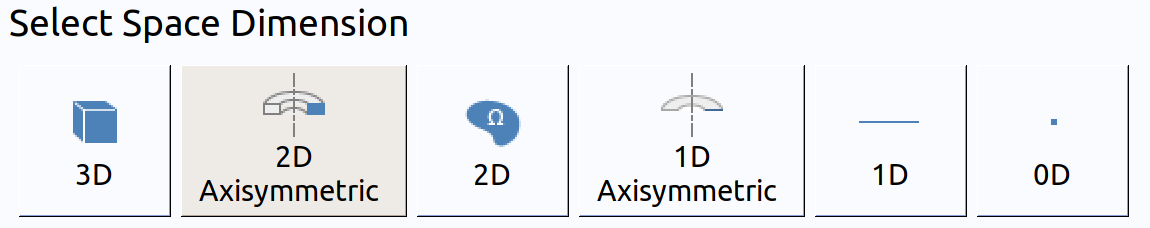
- In the Model Wizard window, click 2D Axisymmetric.
- In the Select Physics tree, select Fluid Flow>Single-Phase Flow>Laminar Flow (spf).
- Click Add.
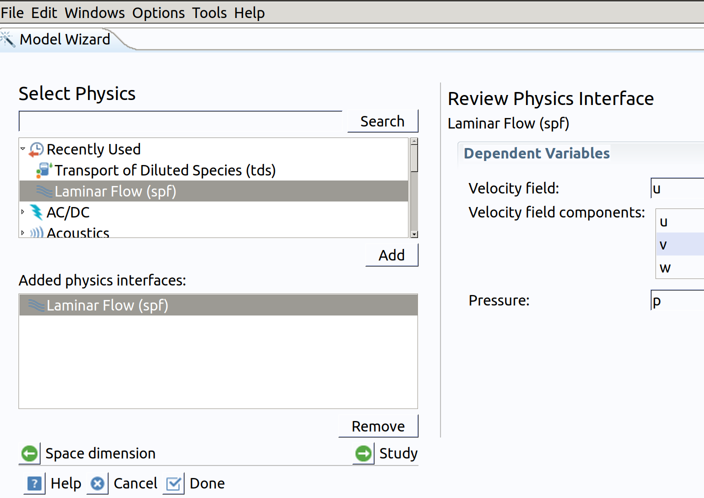
Note: Velocity components are noted: spf.u (along ) and spf.w (along ).
- Click Study.
- In the Select Study tree, select General Studies>Stationary .
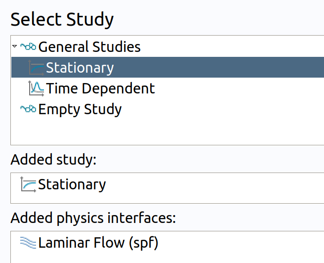
- Go back to Physics.
- In the Select Physics tree, select Chemical Species Transport>Transport of Diluted Species (tds) .
- Click Add.
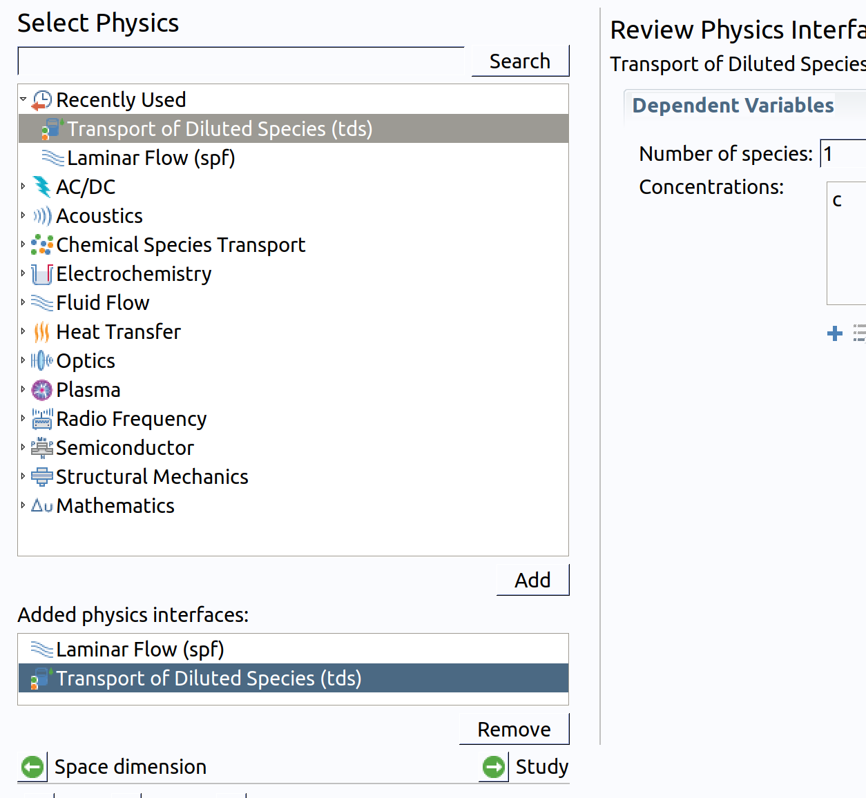
Note: Concentration field will be defined in all domain as c with default units . The additional Time-Dependent problem cannot be set with the wizard
- Click Done.
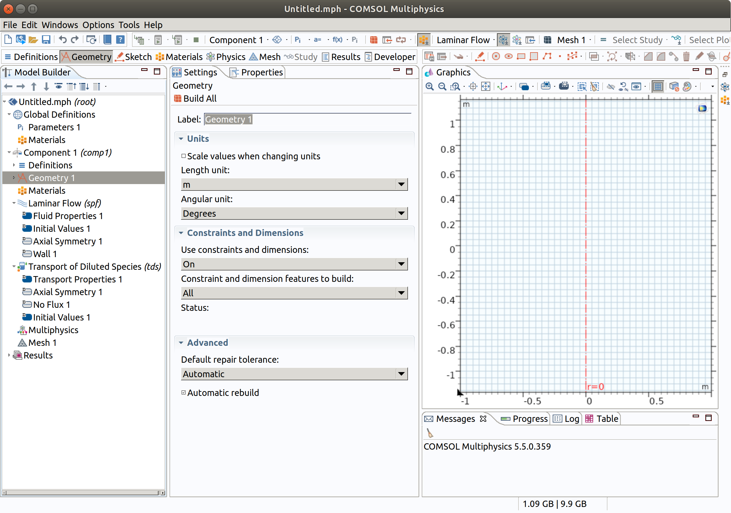
As show on the horizontal bar, it is recommended to complete setting in the following order: Definitions, Geometry, Sketch, Materials, Mesh, Study. At this stage, save your project.
2. GLOBAL DEFINITIONS
- In the Model Builder window, under Global Definitions click Parameters 1 .
- In the Settings window for Parameters , locate the Parameters section.
- Click Load from File .
- Browse to the location of this template and double-click the file hose_parameters.txt.
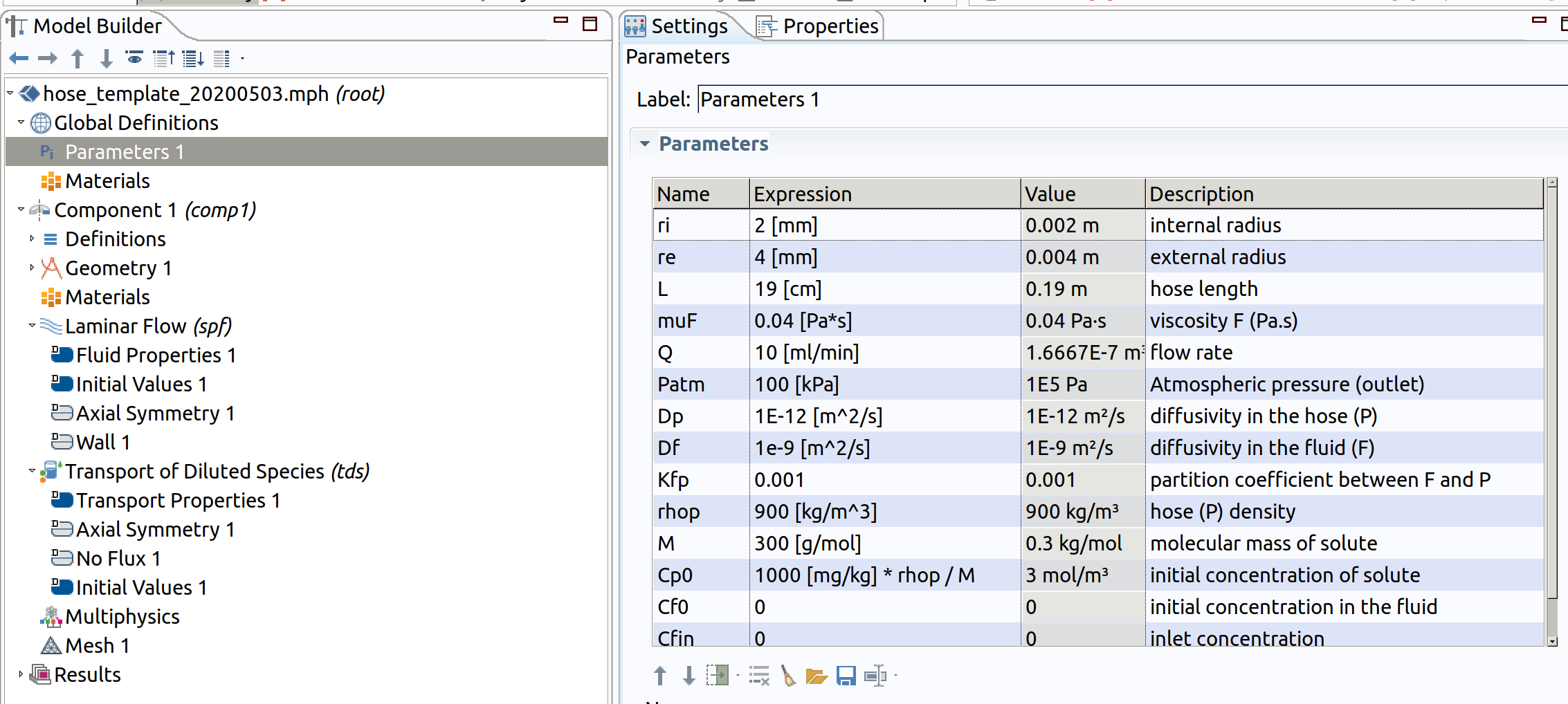
Notations are standard (wit units between [ ]) and are summarized for convenience in Table 1. SI units and mol/volume units are used internally for concentrations.
Table 1. Short description of input parameters.
| Entity | related parameters |
|---|---|
| Hose | radii (, ), length () |
| Circulating liquid | Comsol Multiphysics offers a database of materials (water, olive oil). Most of the properties (density with temperature) can be picked from there. However, some viscosities are missing. I included to fill the gap. |
| Flow | flow rate: , initial/inlet concentrations , , pressure at the end of the hose: (it can be higher than the atmospheric pressure, if the hose is submerged in a liquid) |
| Polymer | denisty: |
| Solute | : molecular mass, diffusivities: , ; partition coefficient (respectively to volume concentrations) |
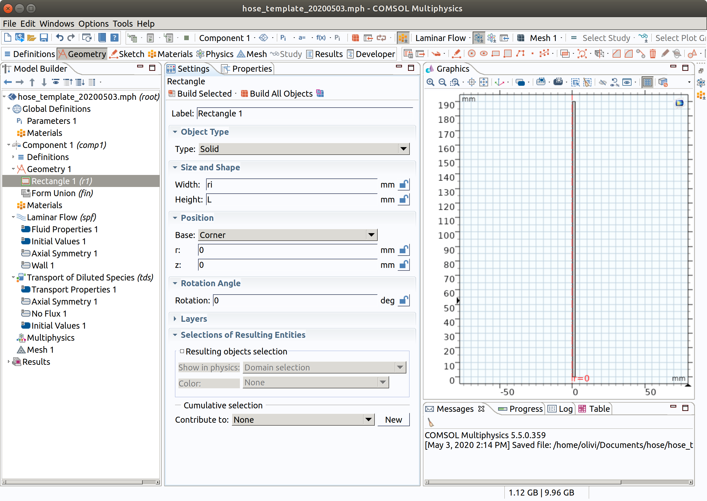
3. GEOMETRY 1
Draw the geometry and make selections.
3.1 Preparation
- In the Model Builder window, under Component 1 (comp1) click Geometry 1 .
- In the Settings window for Geometry , locate the Units section.
- From the Length unit list, choose mm (or keep m, it affects only plots).
3.2 Rectangle 1 (r1)
- In the Geometry toolbar, click Rectangle.
- In the Settings window for Rectangle , locate the Size and Shape section.
- In the Width text field, type ri.
- In the Height text field, type L .
- Click Build Selected .
- Click the Zoom Extents button in the Graphics toolbar.
- Change the Label to inner.
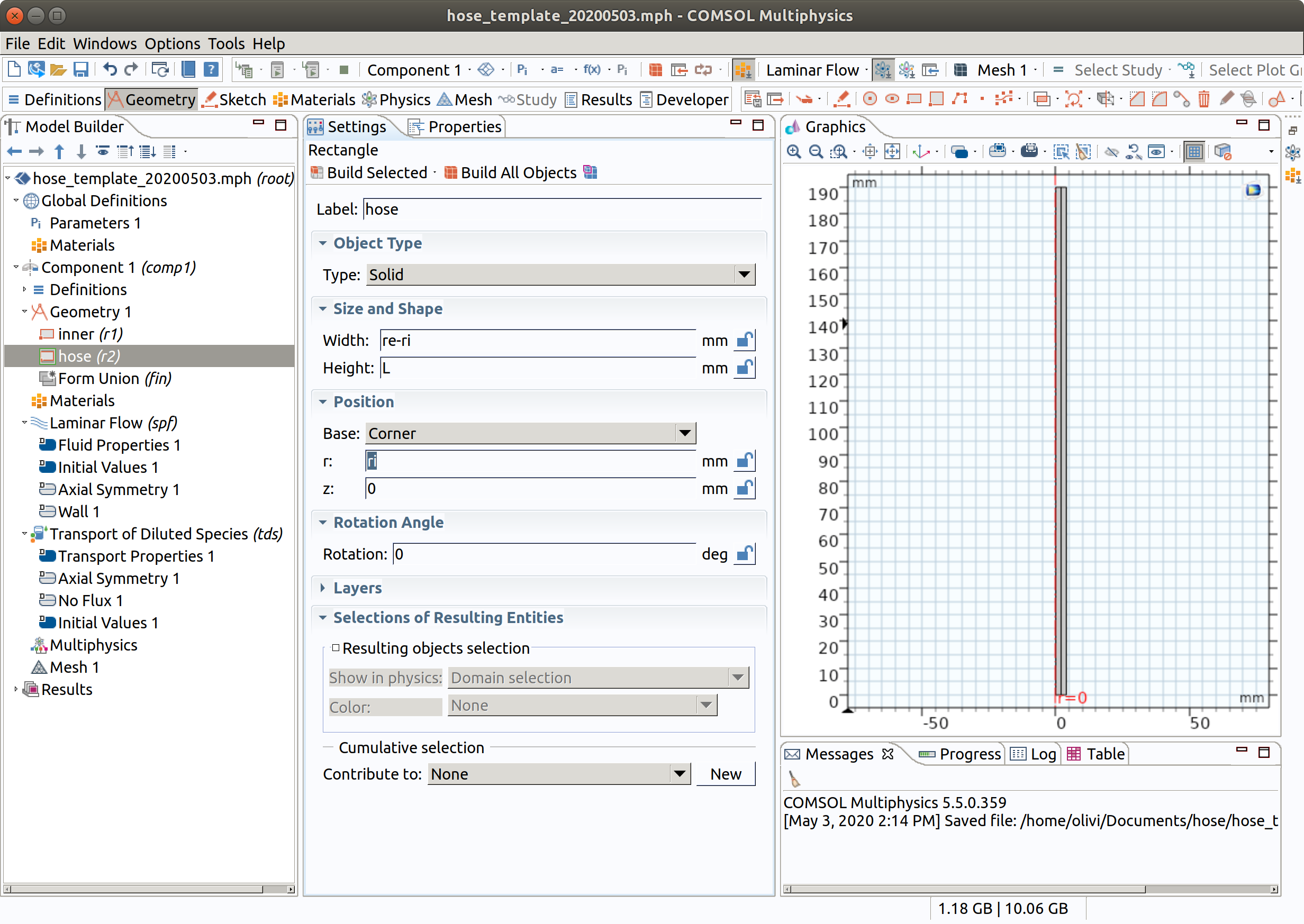
3.3 Rectangle 2 (r2)
- In the Geometry toolbar, click Rectangle.
- In the Settings window for Rectangle , locate the Size and Shape section.
- In the Width text field, type re-ri.
- In the Height text field, type L.
- Locate the Position section. In the r text field, type ri.
- Click Build Selected.
- Click the Zoom Extents button in the Graphics toolbar.
- Change the Label to hose.
4. ADD MATERIAL
4.1 Define the liquid circulating through the hose (inner)
- In the Home toolbar, click Add Material to open the Add Material window.
- Go to the Add Material window.
- In the tree, select Liquids and Gases>Liquids>Olive Oil .
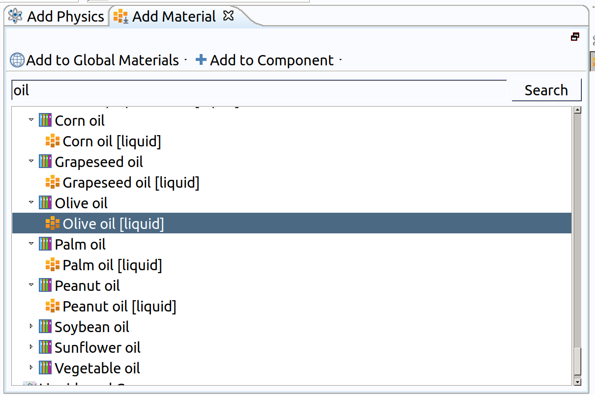
- Click Add to Component in the window toolbar.
- In the Home toolbar, click Add Material to close the Add Material window.
- Set the material active only for domain 1.
- Set the missing viscosity muF.
- Rename the material Food simulant.
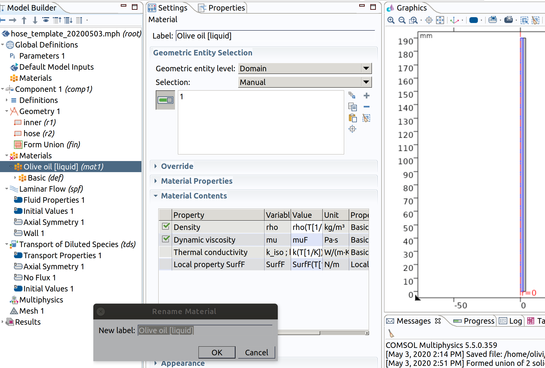
Future modifications (override) of the liquid simulant can be carried out directly in the section Material Contents. Only the properties in connection with the simulated physics are shown.
4.2 Define the properties of the polymer in the hose walls
- In the Home toolbar, click Add Material to open the Add Material window.
- Go to the Add Material window.
- Search for polyethylene (or any other polymer, the Materials library needs to have been installed).
- Click Add Material
- Set the material active only for domain 2.
- Rename the material Polymer.
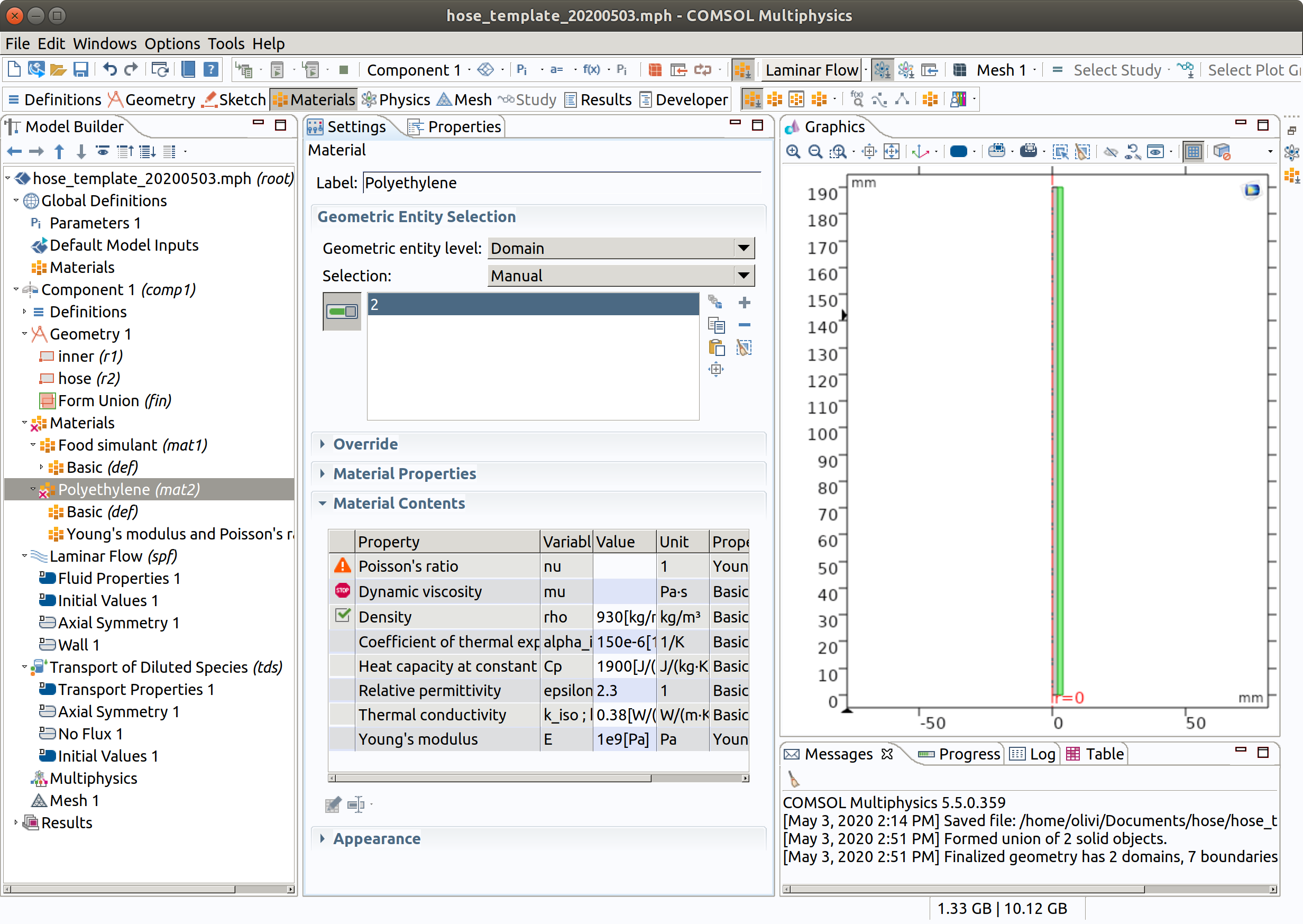
Note that viscosity may be active because we did not restrict the flow to domain 1
5. LAMINAR FLOW (SPF)
5.1 Domain selection and master equation
- In the Model Builder window, under Component 1 (comp1) click Laminar Flow (spf).
- In the Settings window for Laminar Flow , locate the Domain Selection section.
- From the Selection list, remove 2 (hose) and be sure to pick only domain 1 (inner)
- Set Temperature to 313.15 K (standard temperature used in migration testing).
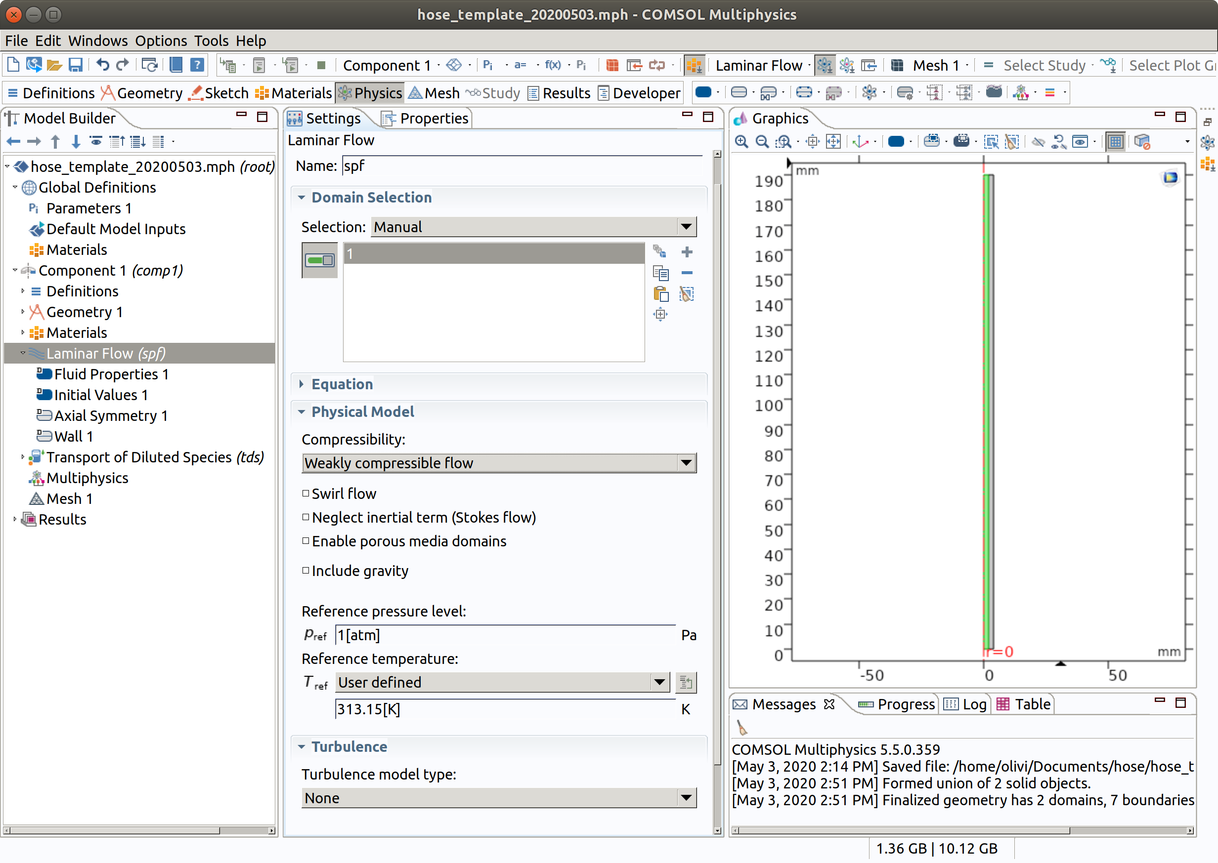
Note that the flow is weakly compressible and that the same model could be used in industrial setups.in
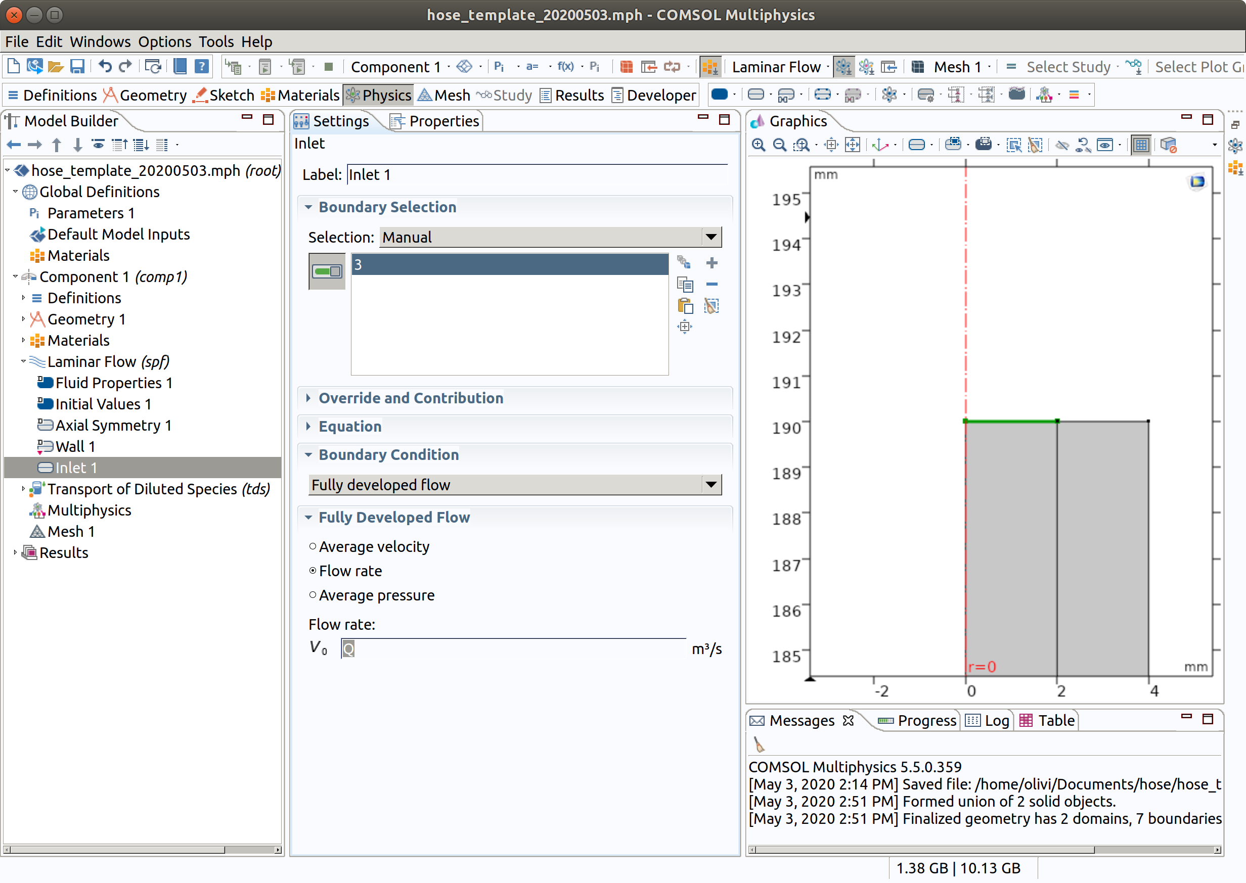
5.2 Inlet
- In the Physics toolbar, click Boundaries and choose Inlet.
- Select Boundary 3 (top) only.
- In the Settings window for Inlet , locate the Boundary Condition section.
- From the list, choose Fully developed flow.
- Locate the Fully Developed Flow section. In the flow rate field (), set Q.
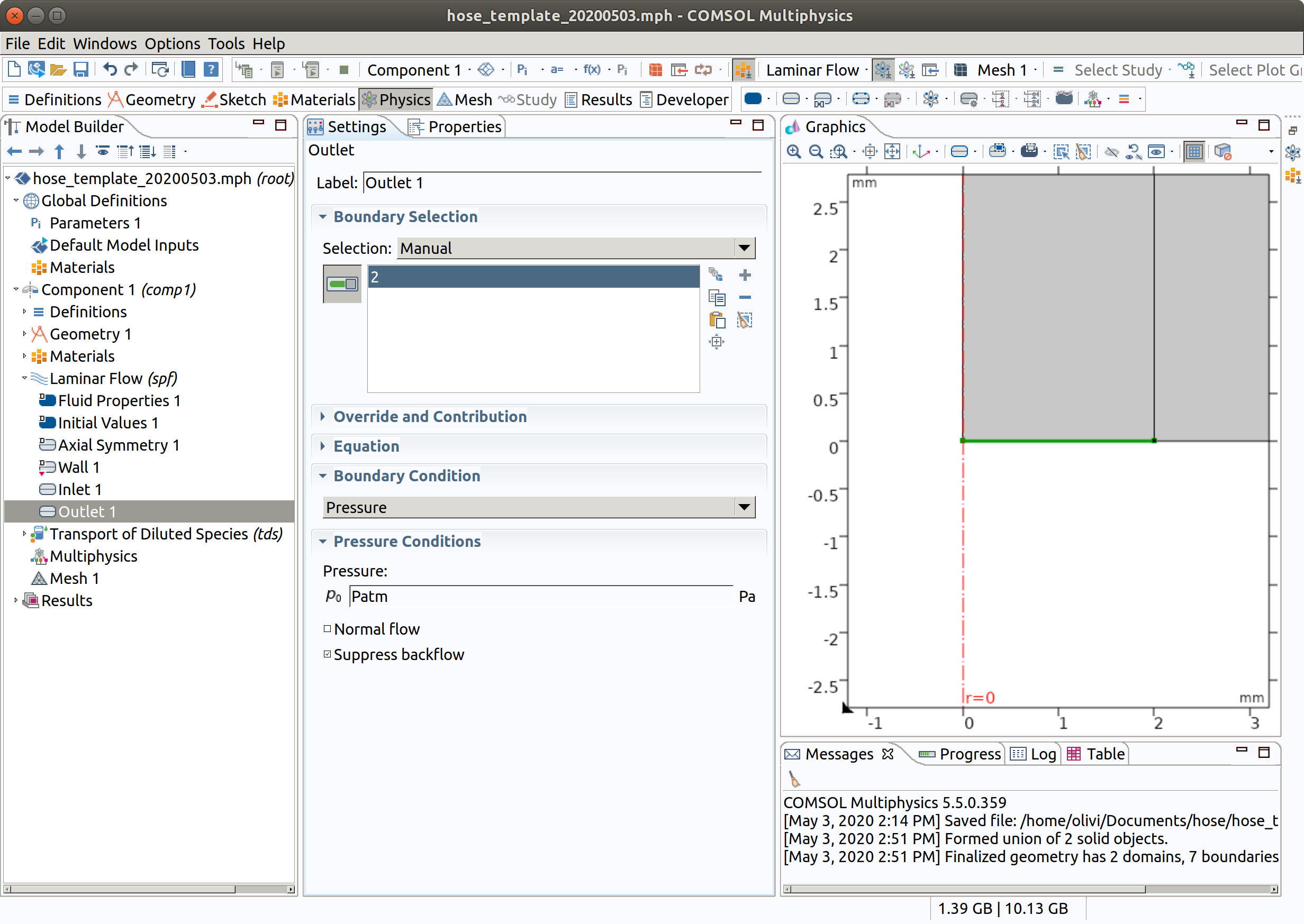
5.3 Outlet
- In the Physics toolbar, click Boundaries and choose Outlet.
- Select Boundary 2 only.
- Set pressure at the boundary equal to Patm
6. SETTING THE PHYSICS OF MIGRATION (tds)
In the Model Builder window, under Component 1 (comp1), choose Transport of Diluted Species (tds)
6.1 Domain selection and master equation
- Check that the domains 1 (inner) and 2 (hose) are selected.
- Since no study has been defined yet, choose time-dependent.
- Verify that convection is checked as transport mechanism
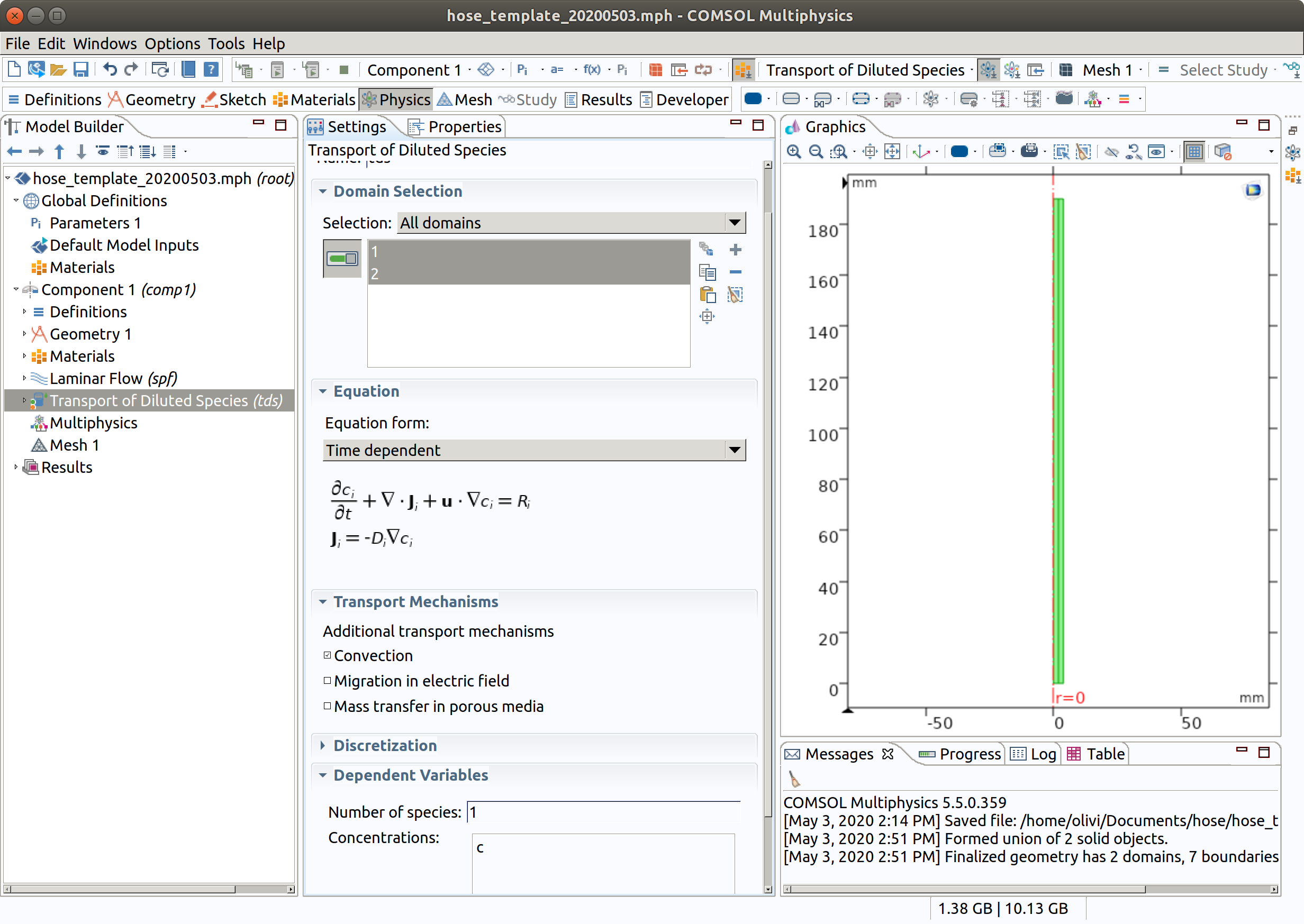
Note that we have only one single species, but several could be added.
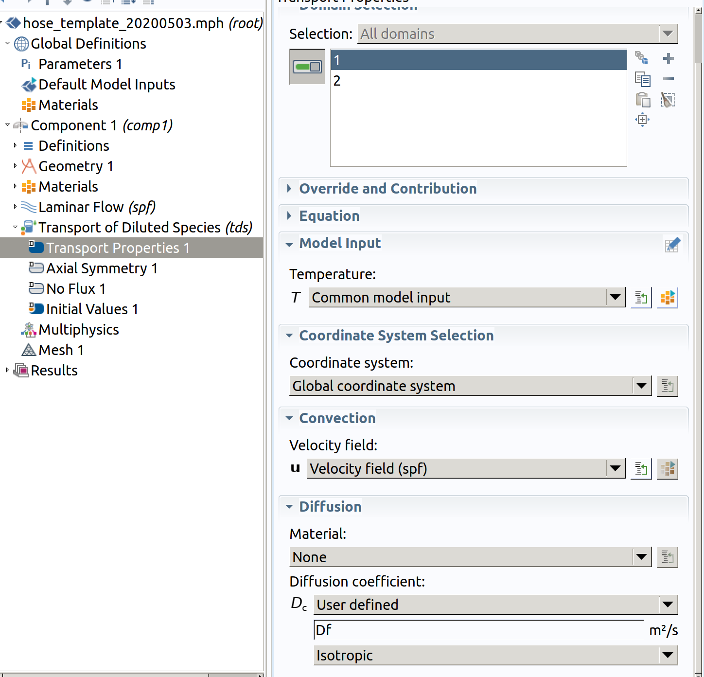
6.2 Transport properties 1 (initially for domains 1 and 2)
- In the Physics toolbar, select Transport properties 1 (you cannot restrict the properties to a specific domain at this stage).
- Select spf as velocity field
- Type Df as diffusion coefficient.
6.3 Transport properties 2 (override for domain 2 hose)
- In the Physics toolbar, right click on Transport of Diluted Species, add Transport properties
- Select domain 2 (hose)
- Type Dp as diffusion coefficient
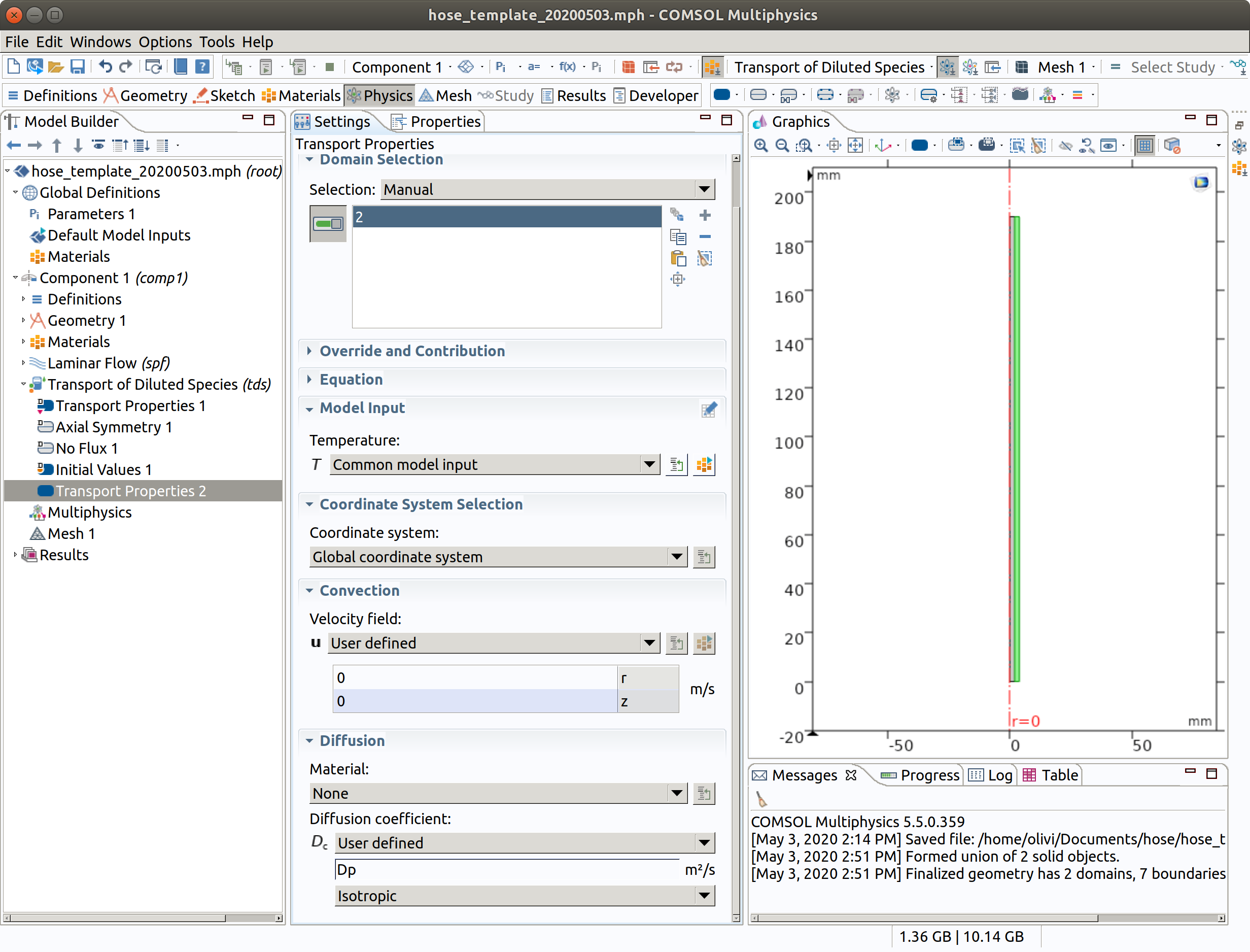
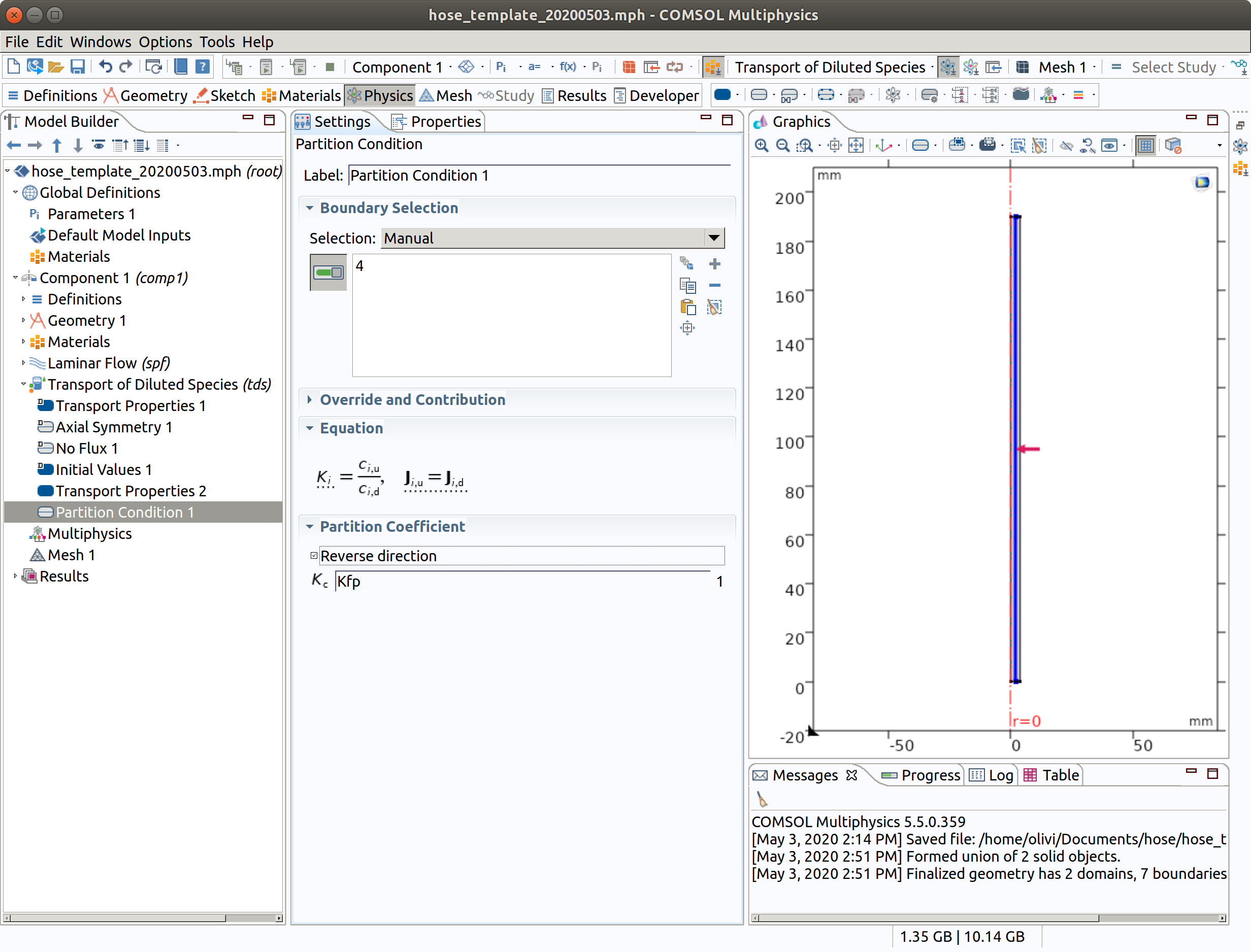
6.4 Partition condition (between 2 hose and 1 inner)
- In the Physics toolbar, right click on Transport of Diluted Species, add Partition condition
- Select boundary condition 4
- Type Kfp as partition coefficient
- Check reverse direction
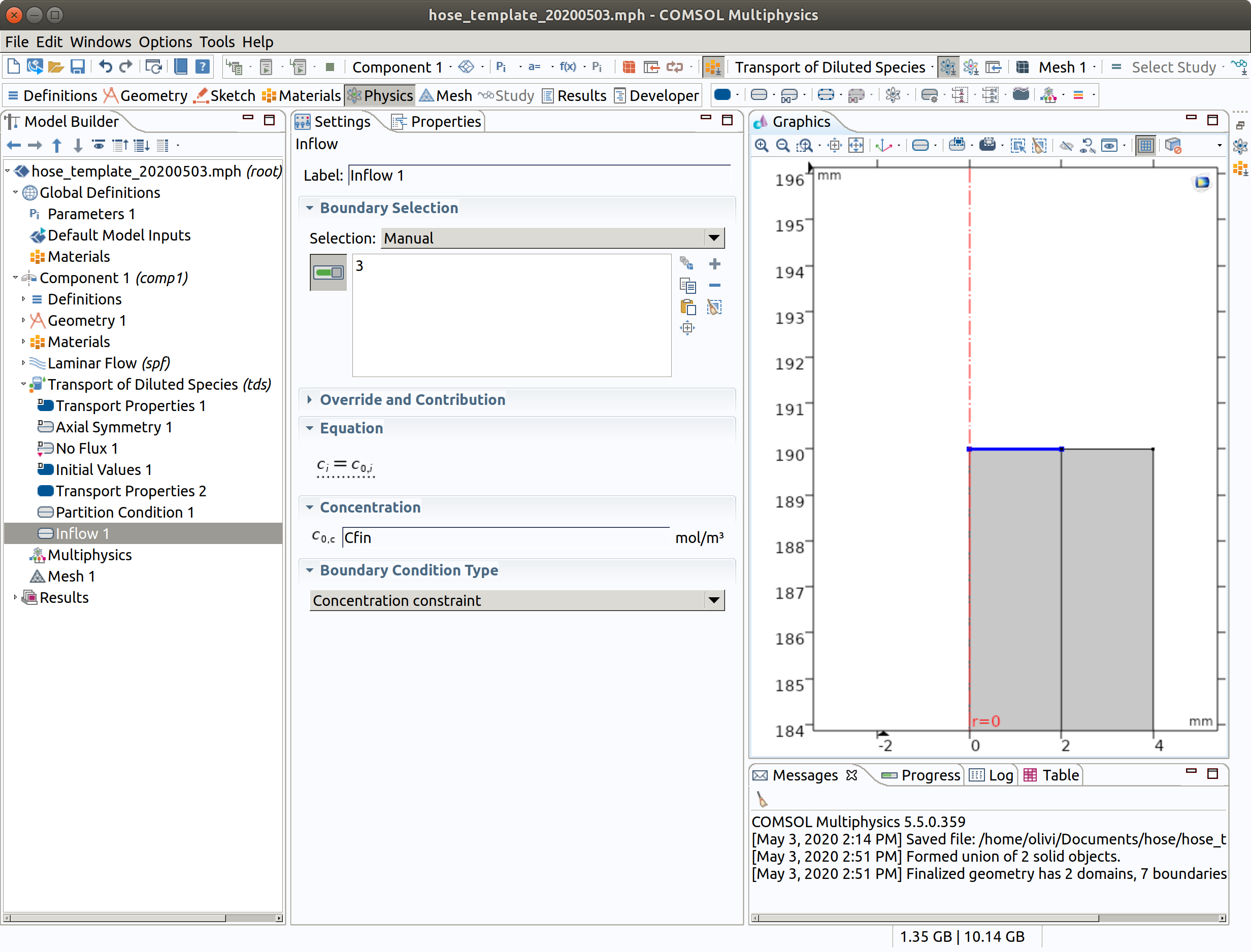
6.5 Inflow 1
The inflow may contain some amount of migrants (e.g., connected pipes)
- In the Physics toolbar, right click on Transport of Diluted Species, add Inflow.
- Select boundary condition 3.
- Type Cfin as inflow concentration
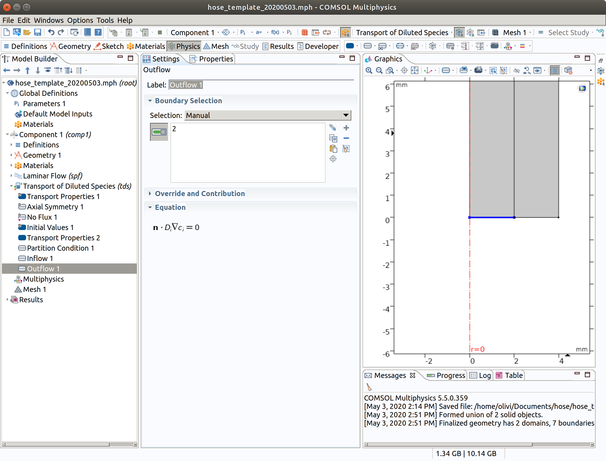
6.6 Outflow 1
The outflow is a free flow such as if the leaving liquid was pouring without contact in a beaker/recipient.
- In the Physics toolbar, right click on Transport of Diluted Species, add Outflow.
- Select boundary condition 2
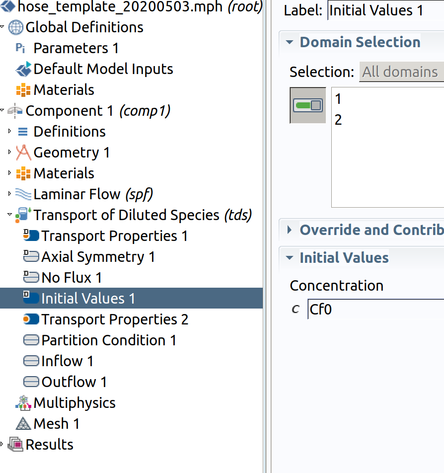
6.7 Initial Values 1 (default value for 1 innerand 2 hose)
- Type Cf0 as initial values
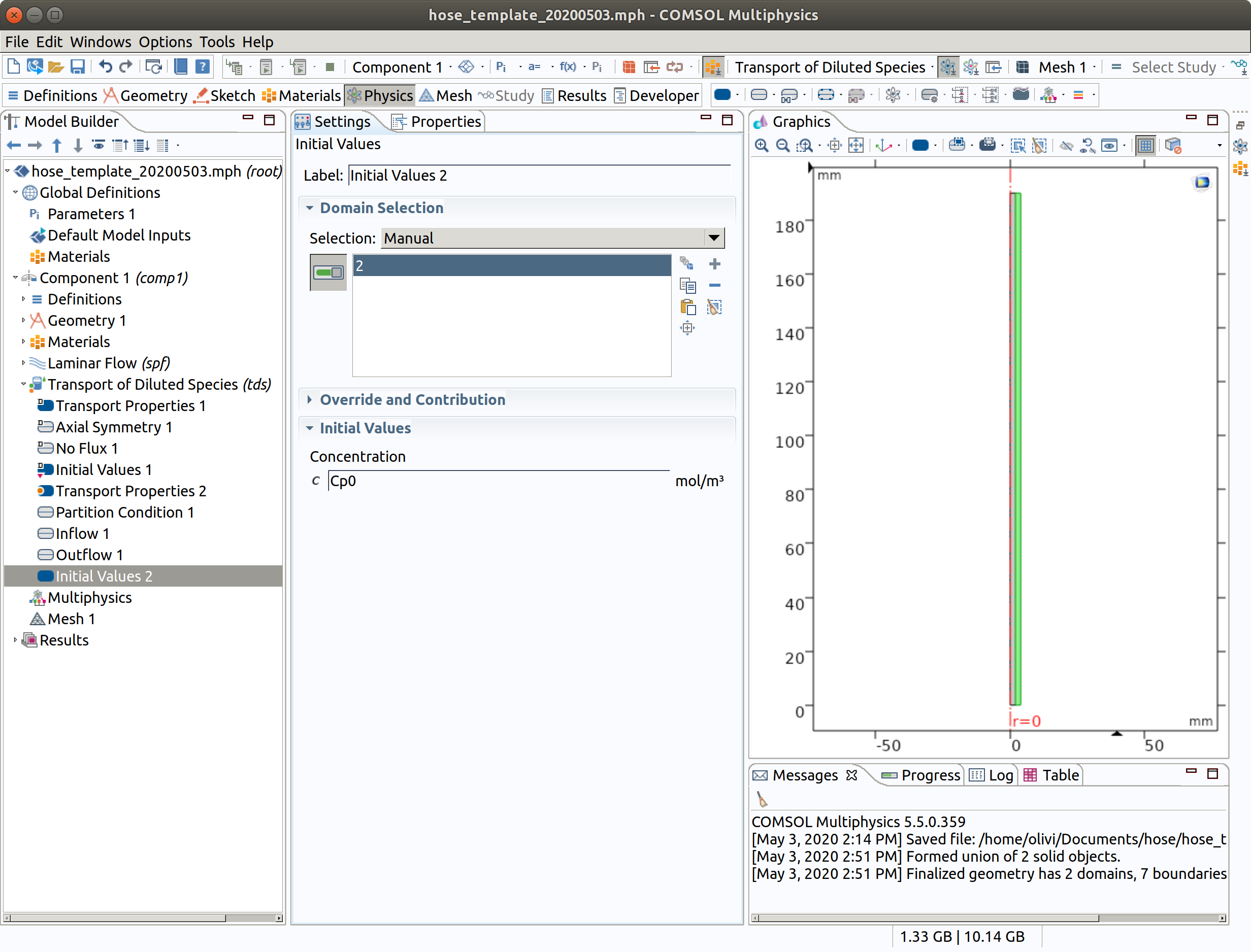
6.8 Initial Values 2 (override for for 2 hose)
- In the Physics toolbar, right click on Transport of Diluted Species, add Initial Values.
- Select domain condition 2 (hose)
- Type Cp0 as **initial concentration.
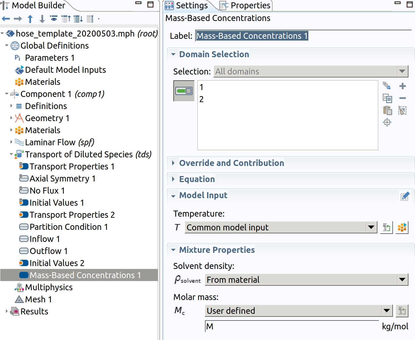
6.9 Mass-Based Concentrations 1
This step enable to get mass concentration available (). Mass concentration will be available as tds.cmass_c.
- Type M as Molar Mass
7. Setting MESH: Mesh 1
A mapped mesh is required for stability and efficiency. Do not use triangular mesh.
7.1 Mapped 1 (1 inner)
In the Model Builder window, under Component 1 (comp1) right-click Mesh 1 and choose Mapped .
Select domain 1 (inner).
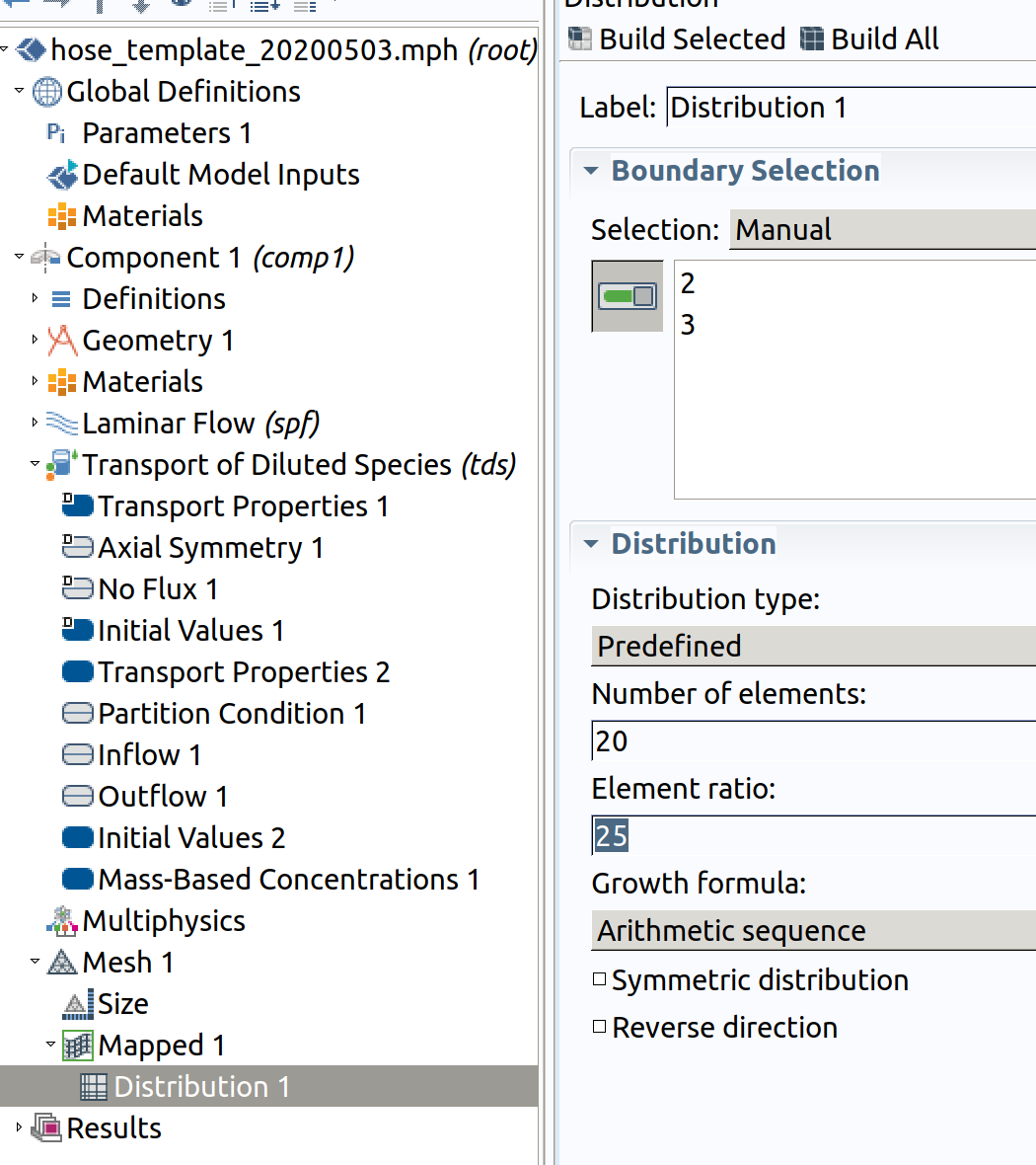
Distribution 1 (resolution along )
- In the Model Builder window, right-click Mapped 1 and choose Distribution.
- Select Boundaries 2 and 3 only.
- In the Settings window for Distribution , locate the Distribution section.
- From the Distribution type list, choose Predefined.
- In the Number of elements text field, type 20.
- In the Element ratio text field, type 25.
Distribution 2 (resolution along )
- In the Model Builder window, right-click Mapped 1 and choose Distribution.
- Select Boundaries 1 and 4 only.
- In the Settings window for Distribution , locate the Distribution section.
- From the Distribution type list, choose Number of elements of elements.
- In the Number of elements text field, type 50 .
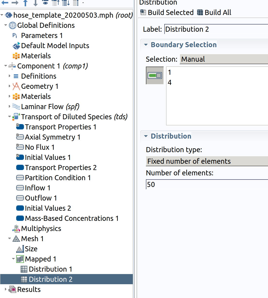
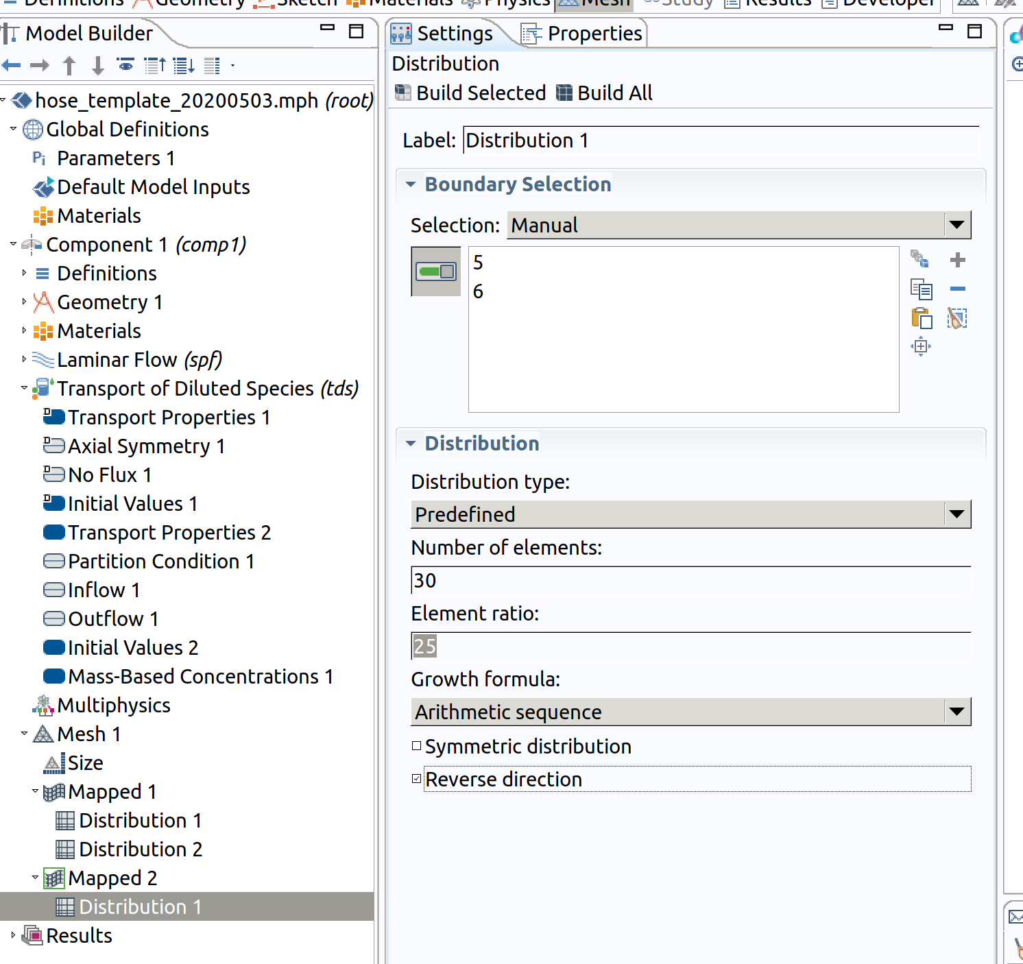
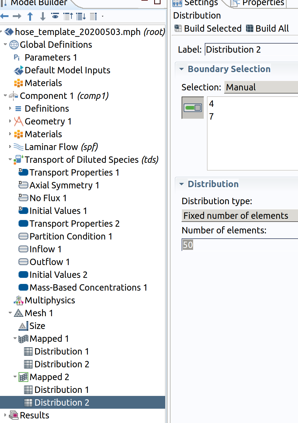
7.2 Mapped 2 (2 hose)
In the Model Builder window, under Component 1 (comp1) right-click Mesh 1 and choose Mapped .
Select domain 1 (hose) or choose remaining.
Distribution 1 (resolution along )
- In the Model Builder window, right-click Mapped 1 and choose Distribution.
- Select Boundaries 5 and 6 only.
- In the Settings window for Distribution , locate the Distribution section.
- From the Distribution type list, choose Predefined.
- In the Number of elements text field, type 30.
- In the Element ratio text field, type 25.
- Check reverse order direction (we need a good resolution towards inner).
Distribution 2 (resolution along )
- In the Model Builder window, right-click Mapped 1 and choose Distribution.
- Select Boundaries 1 and 4 only.
- In the Settings window for Distribution , locate the Distribution section.
- From the Distribution type list, choose Number of elements of elements.
- In the Number of elements text field, type 50 .
8. STUDY 1
If Study 1 is not visible in the Model Builder Window, right click on the root node (with filename, the node hose_template in the image above) and add Study>Stationary.
Step 1: Stationary (spf)
- In the Model Builder window, under Study 1 click Step 1: Stationary.
- In the Settings window for Stationary , locate the Physics and Variables Selection section.
- In the table, clear the Solve for check box for Transport of Diluted Species (tds), keep only spf.
- In the Study toolbar, click Compute .
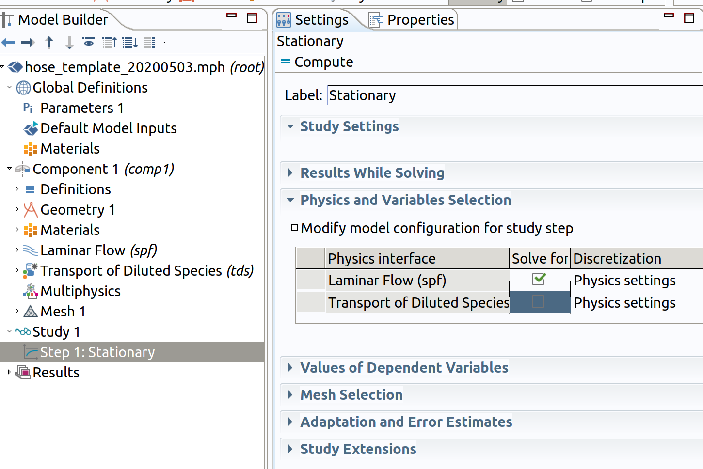
Clearing Transport of Dilutes Species remove the definitions of tds during the resolution of spf at steady-state.
9. STUDY 2
Add Study 2 by clicking on the root node (with filename, the node hose_template in the image above) Study>TIme Dependent.
Step 1: Time Dependent (tds)
- In the Study toolbar, click Study Steps and choose Stationary>Time dependent.
- Choose min as Time unit.
- Enter ({range(0,0.05,sqrt(10000))})^2 as Times to mimic diffusion time scale.
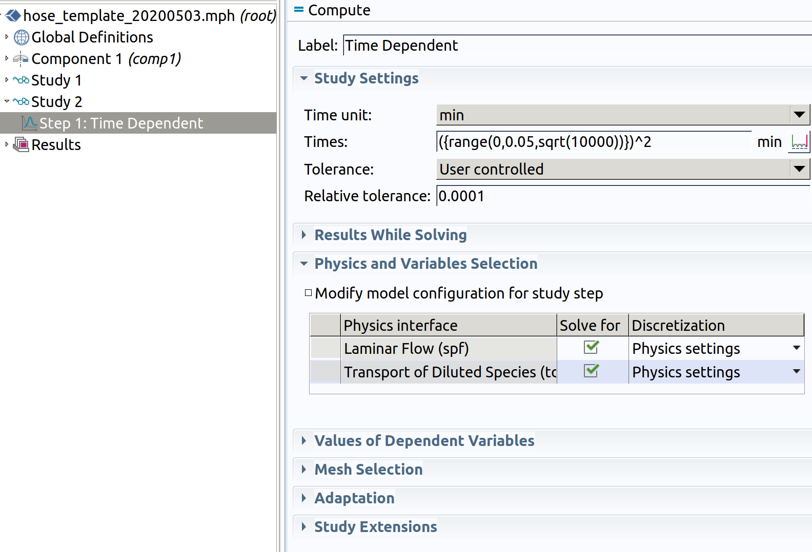
Keep spf, if not the velocity flow will not be available to calculate tds.
10. PROBES
We need probes and additional variables to retrieve easily results.
The preferred quantity to understand mass transfer (migration) under various flow conditions is amount of transferred substance in or .
10.1 Boundary Probe 1
In the Model Builder window, go to Component 1 (comp1) > Definitions and choose Probes >Boundary Probe.
- Type migration rate as label.
- Type Jmig as name.
- Choose Integral as Probe Type.
- Select Boundary 2 only.
- Enter -tds.tflux_cz*M as Expression.
- Keep checked Compute surface integral (as we use cylindrical coordinate system, the expression will be multiplied by ).
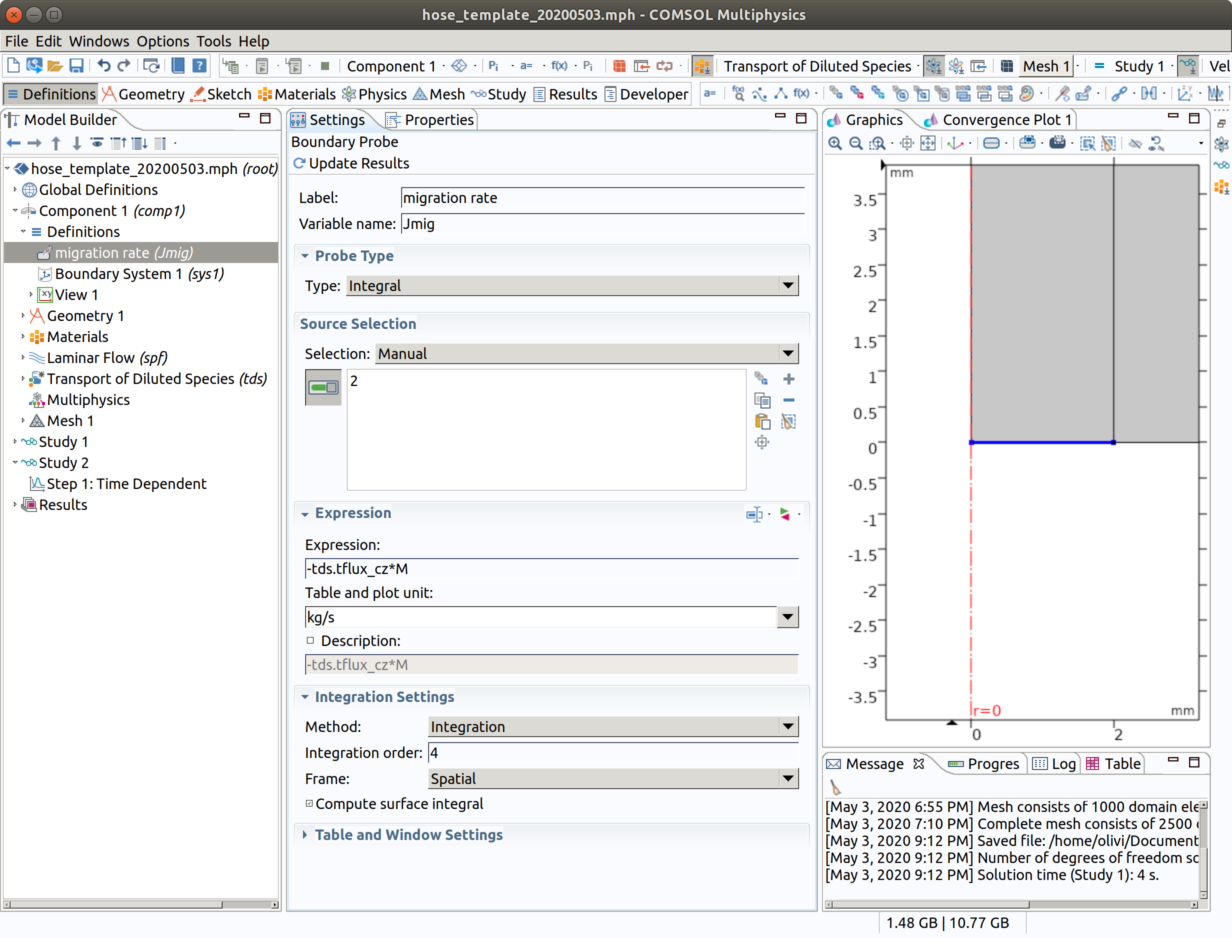
TIP: Probes will be plotted during integration of PDE system. The names of available internal variables can be listed with the tool with the two triangles (red and green) near the Expression title. -tds.tflux_cz is the total (convective+diffusive flux) along .
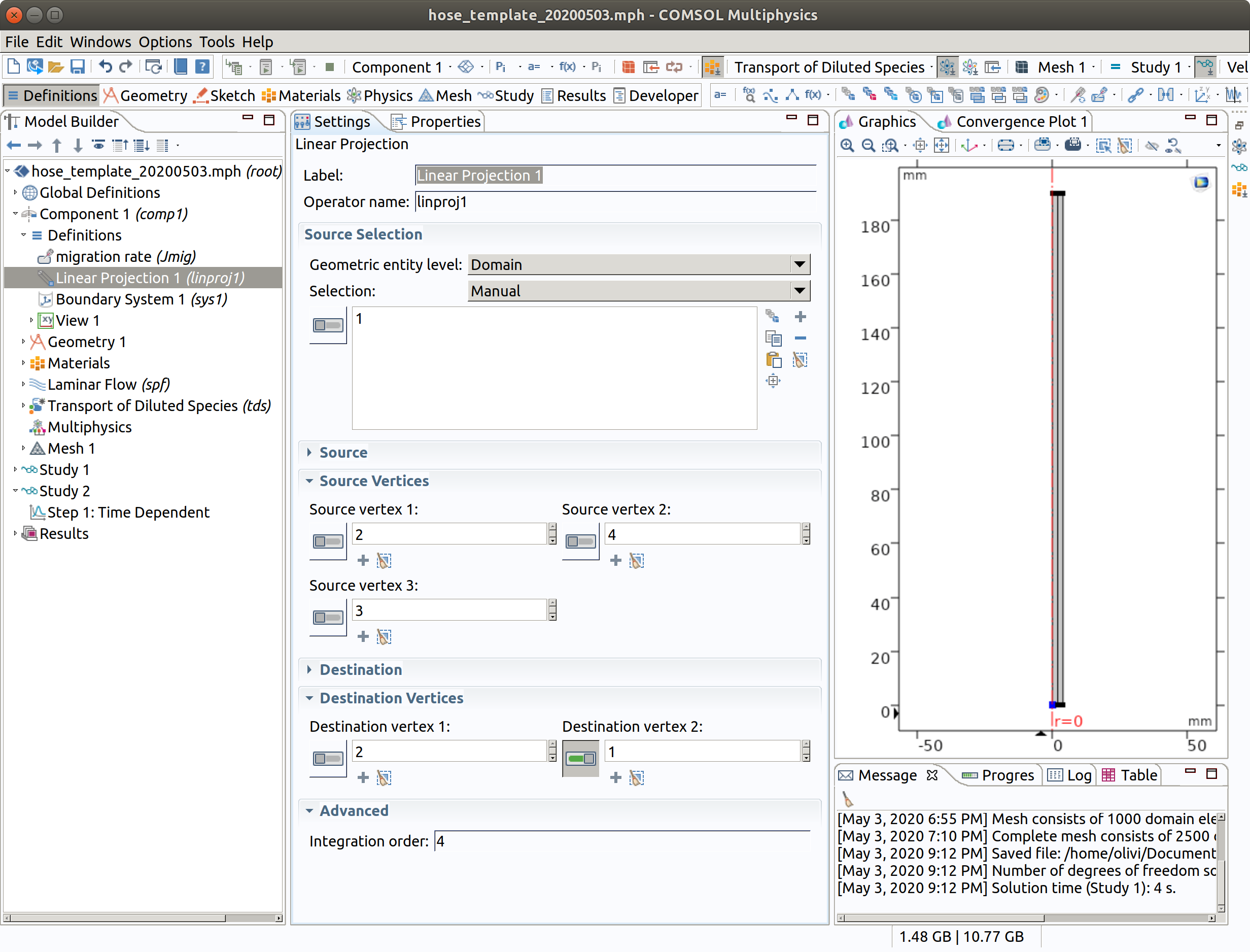
10.2 Linear Projection 1
Projection is used to get the linear profile along the hose. The projection is defined from a source plane (defined by 3 vertices) onto a line (defined by 2 vertices). The so-defined is operator will be available as linproj1() in subsequent calculations.
In the Model Builder window, go to Component 1 (comp1) > Definitions and choose Non Local Couplings >Linear Projection.
- Select domain 1 (inner).
- Pick 2,4,3 as Source Vertices.
- Pick 2,1 as Destination Vertices.
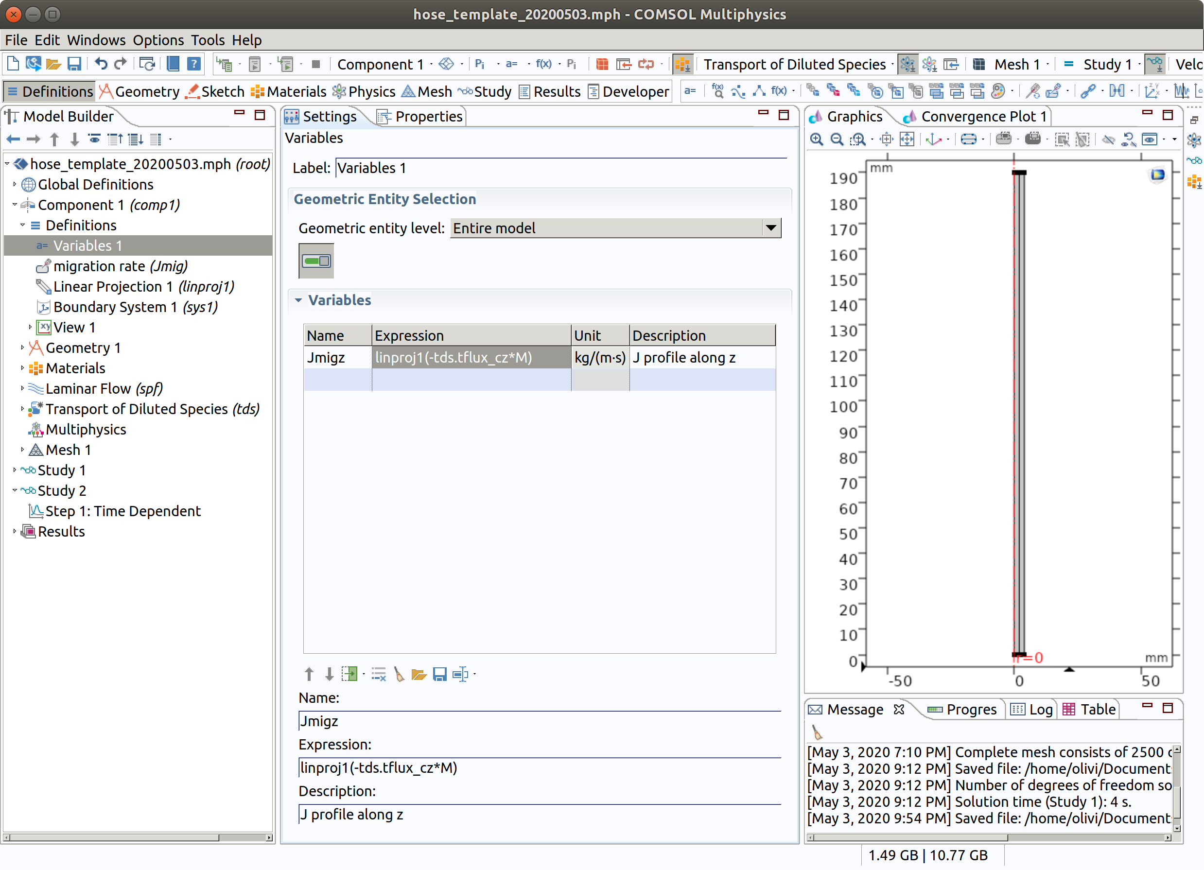
10.3 Variables 1
A new variable Jmigz is created and will be available for post-processing and plotting. It is defined as the amount of substance crossing the hose at the position . Note that this amount is originating from all the positions above and in a less extent (negligible) from below by diffusion.
In the Model Builder window, go to Component 1 (comp1) > Definitions and choose Variables.
- Type Jmigz as label.
- Enter linproj1(-tds.tflux_cz*M) as Expression.
- Type J profile along z as Description.
11. RUN Study 2
- Run once Study 1 if you forget.
- Run Study 2.
During calculations, probe 1 (migration rate) is shown as well as tabulated values. The calculations are completed in 24 s on .
Default plots are generated at the end of the simulation.
12. POST-PROCESSING
Plot concentration profiles along lines.
12.1 Cut Line 2D 1 (middle)
In the Model builder window, go to Results>Datasets and create a Cut Line 2D 1
- Type middle as label.
- Choose Study2/.... as Dataset.
- Type 0 and L/2 for Point 1.
- Type ri+re and L/2 for Point 2.
12.2 Cut Line 2D 1 (outlet)
Duplicate the line middle, to create a similar line at the outlet of the hose.
- Type outlet as label.
- Choose Study2/.... as Dataset.
- Type 0 and 0 for Point 1.
- Type ri+re and 0 for Point 2.
Note that this line is also available as a boundary.
12.3 Cut Line 2D 1 (inlet)
Duplicate the line middle, to create a similar line at the outlet of the hose.
- Type inlet as label.
- Choose Study2/.... as Dataset.
- Type 0 and L for Point 1.
- Type ri+re and L for Point 2.
Note that this line is also available as a boundary.
12.4 Cut Line 2D 1 (axis)
Duplicate the line axis, to create a vertical line along the vertical axis of the hose.
1 Type axis as label. 2 Choose Study2/.... as Dataset. 3 Type 0 and L for Point 1. 4 Type 0 and 0 for Point 2.
Note that this line is also available as a boundary.
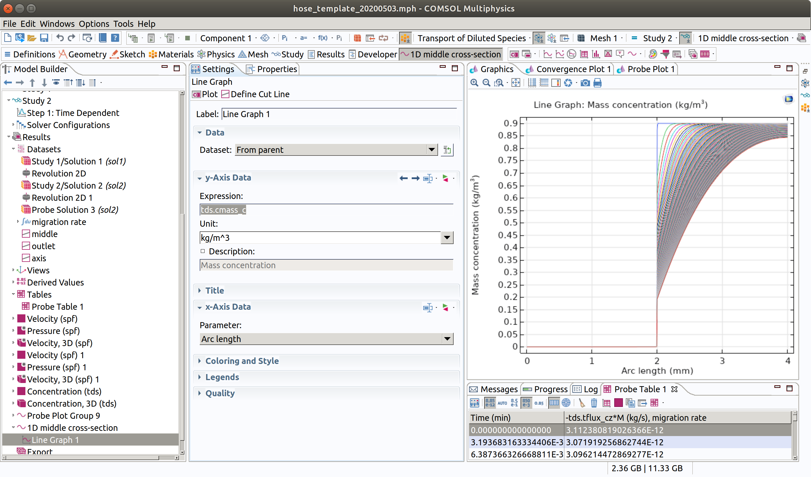
12.5 1D plot group for middle
In the Model builder window, go to Results and create a 1D plot group
1 Type 1D middle cross-section as label. 2 Choose middle as Dataset. 3 Choose Interpolated as Time Selection 4 Type range(0,100,10000) as Times.
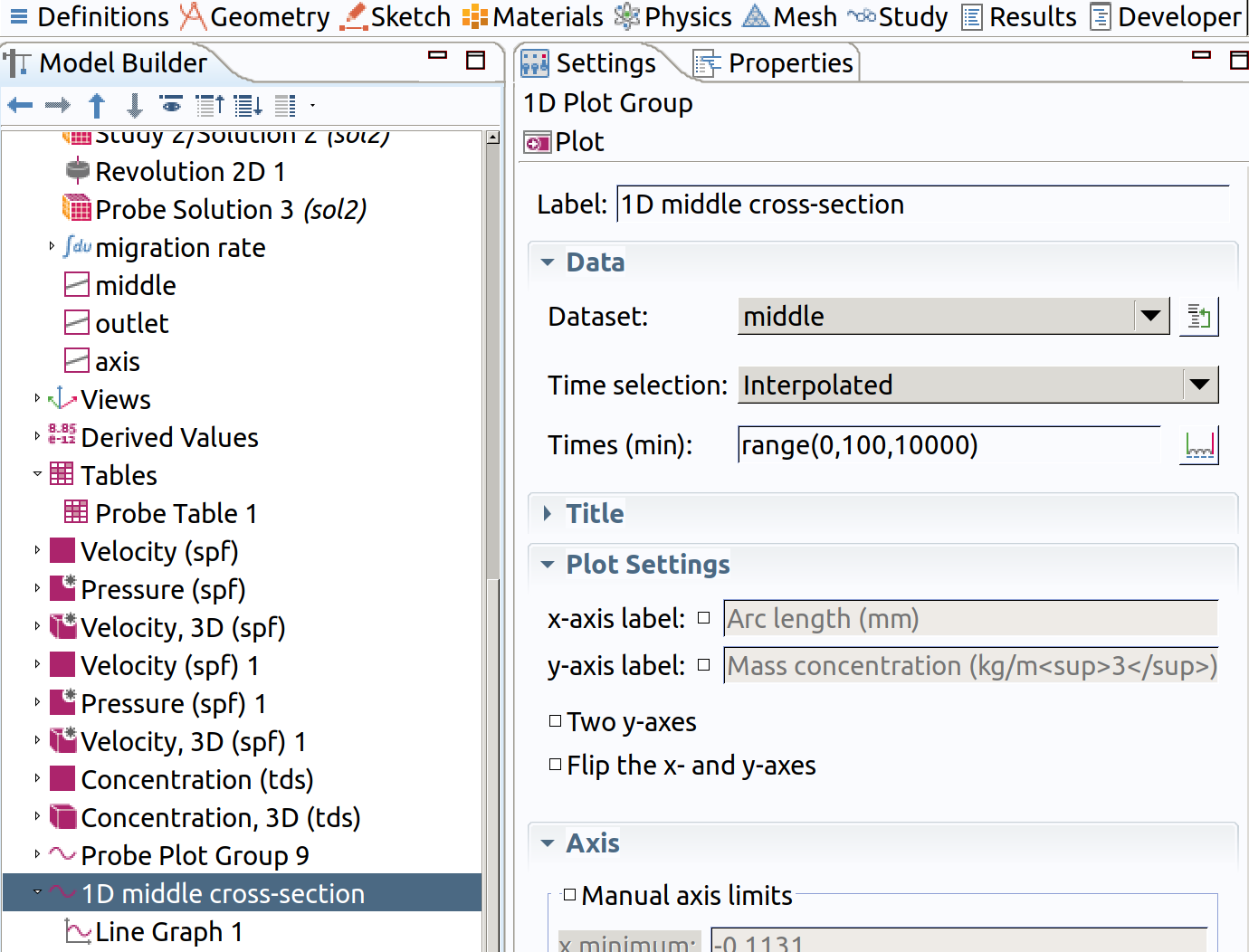
5 Add a line graph in Results>1D middle cross-section 6 Type tds.cmass_c as expression 5 Click plot (top left icon in the settings section)
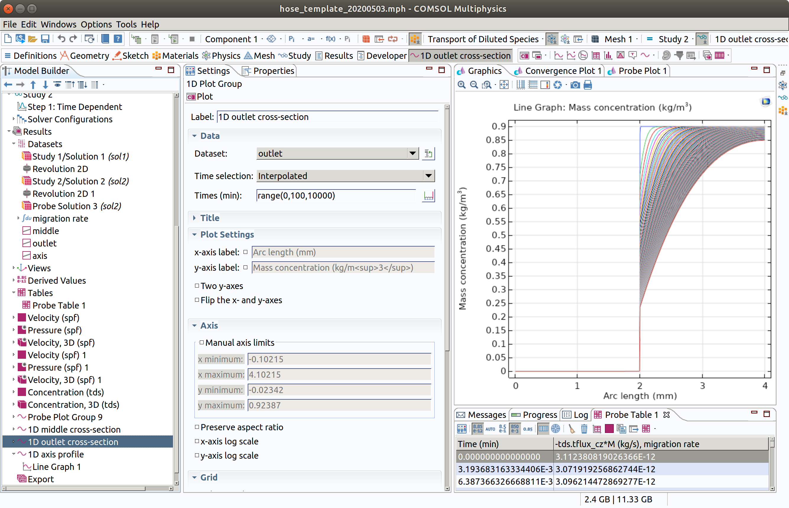
12.6 1D plot group for outlet
Duplicate (right click) the previous group 1D outlet cross-section.
- Type 1D outlet cross-section as label.
- Choose outlet as Dataset.
- Click plot (top left icon in the settings section)
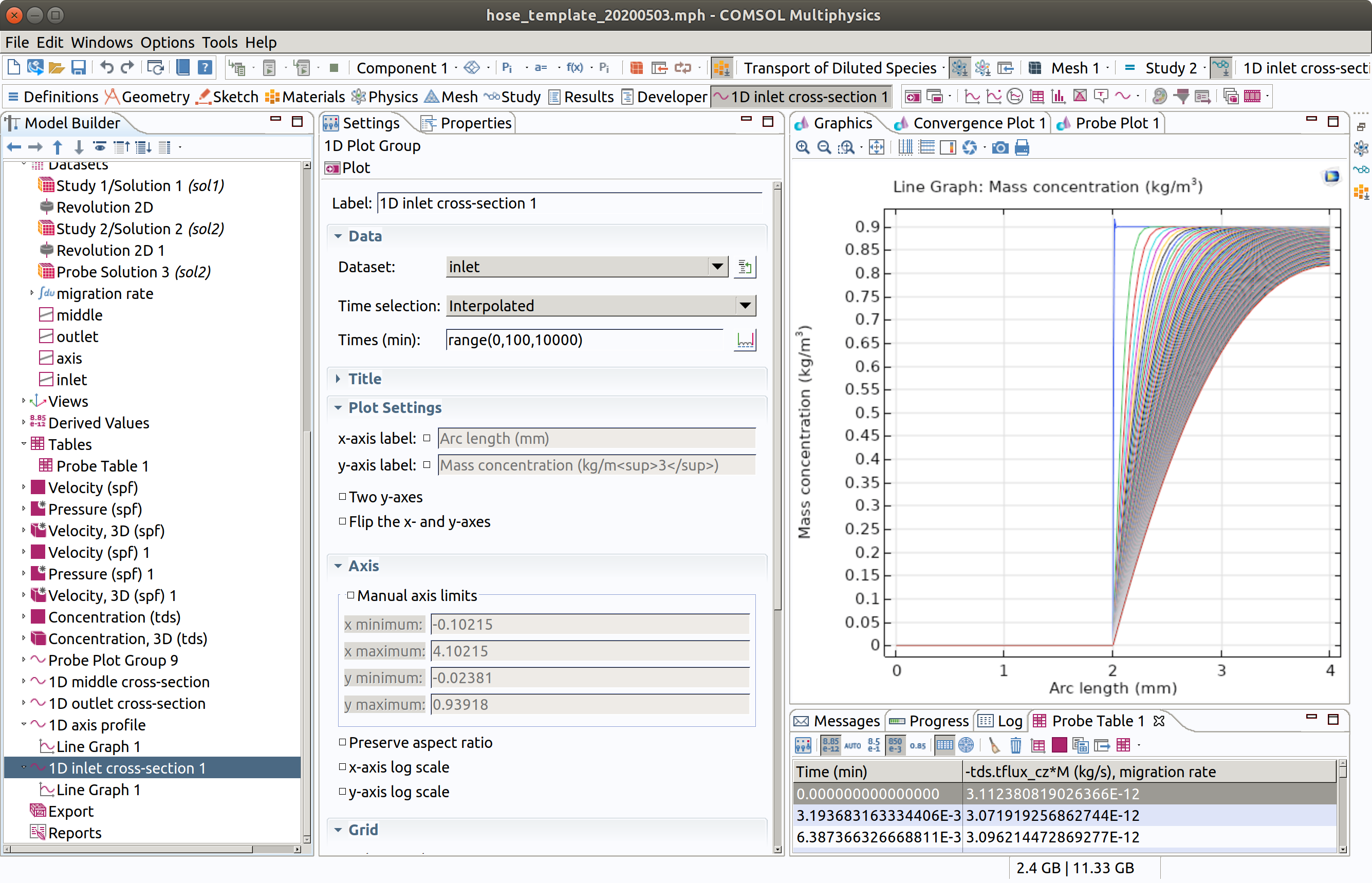
12.7 1D plot group for inlet
The differences between middle and outlet are very small but now look at inlet profiles.
Duplicate (right click) the previous group 1D outlet cross-section.
- Type 1D inlet cross-section as label.
- Choose inlet as Dataset.
- Click plot (top left icon in the settings section)
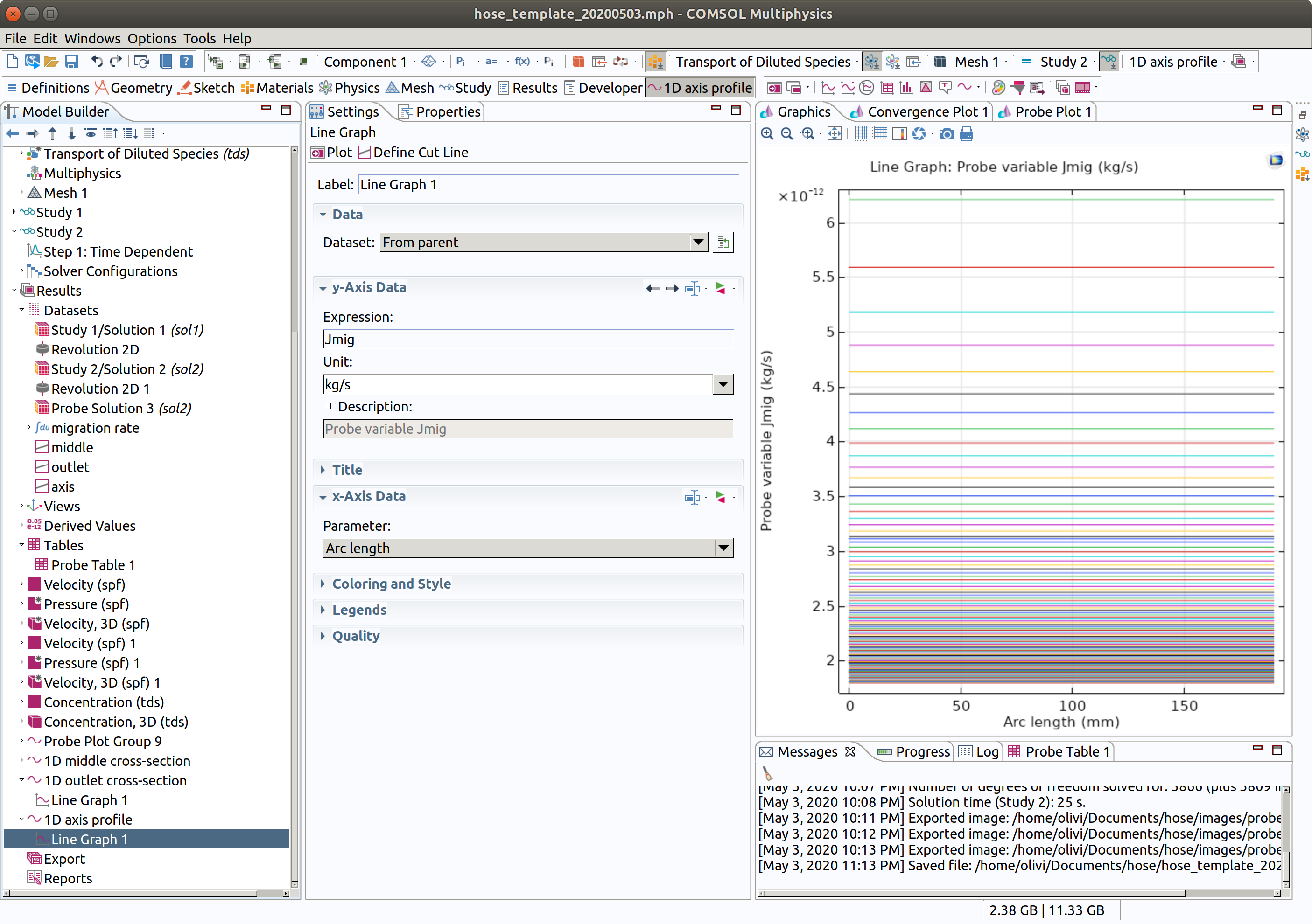
12.8 1D plot group for axis
In the Model builder window, go to Results and create a 1D plot group
- Type 1D axis profile as label.
- Choose axis as Dataset.
- Choose Interpolated as Time Selection
- Type range(0,100,10000) as Times.
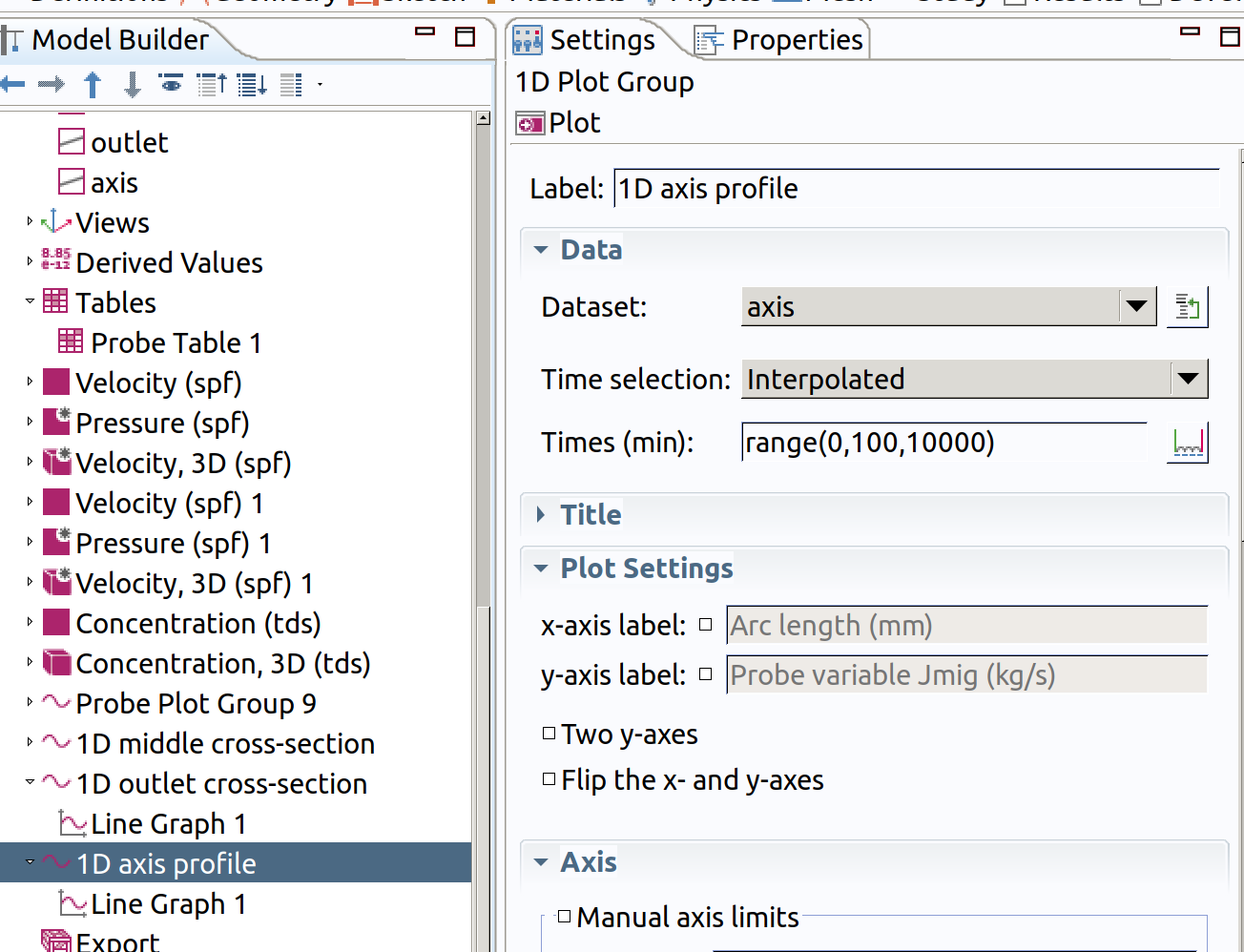
- Add a line graph in Results>1D axis cross-section
- Type Jmig as expression
- Click plot (top left icon in the settings section)
13. PLOT VELOCITY PROFILE
In the Model builder window, go to Results and create a 1D plot group
- Type 1D Velocities as label.
- Choose Study 1/Sol.... as Dataset.
- Add a line graph in Results>1D Velocities
- Select boundary 2 (outlet).
- Type spf.U as expression.
- Check reversed arc length (boundaries are oriented; by reversing it the interface is on the right).
- Click plot (top left icon in the settings section)
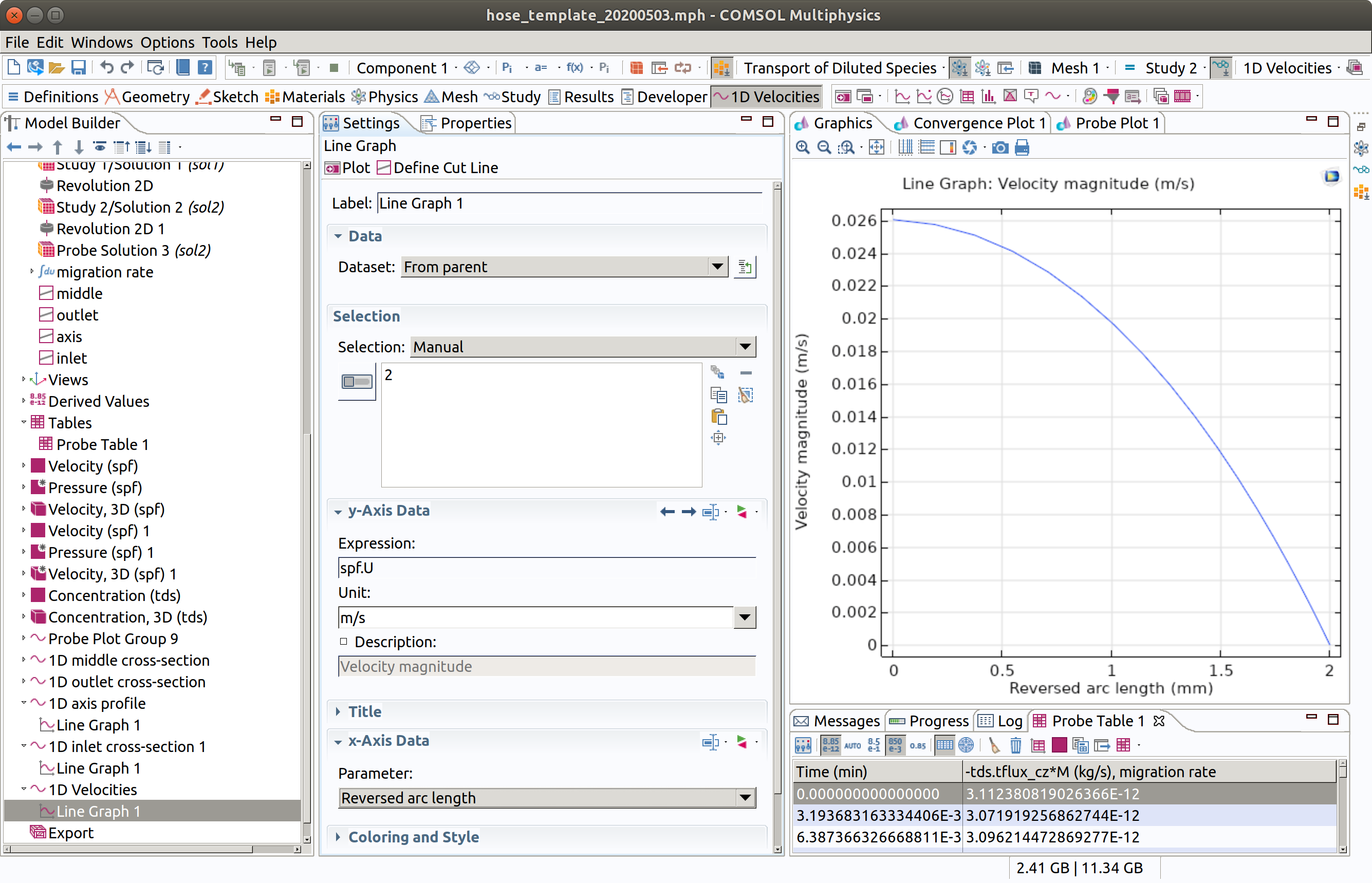
We check that the profile is parabolic.
14. SENSITIVITY ANALYSIS
Calculations are really fast and many configurations can be tested. The problem simulated here is known as Graetz problem. It is particularly useful to understand as a 1D model including a mass transfer resistance at the boundary can achieve similar results or at least overestimate previous results.
Further discussion pending.
In further analyses, it is encouraged to introduce the Graetz number, whose reciprocal value expresses the relative distance from the entrance/inlet, where mass transfer are affected by the flow. Beyond this value, the concentration profiles are fully developed (i.e., the length of the mass boundary layer ).
As a rule of thumb, the concentration profiles can be considered fully developed as soon as or better .
15. EXPLORATION WITH MATLAB
15.1 Launch Matlab with Comsol as a server
For a Linux installation, type:
xxxxxxxxxxcomsol mphserver matlabFor a Windows or Mac installation, look for the shortcut icon
COMSOL Multiphysics with MATLABor via the Windows start menu underAll Programs>COMSOL Multiphysics 5.5>COMSOL Multiphysics 5.5 with MATLAB.On Mac OS X, use the
COMSOL with MATLABapplication available in theApplicationfolder
15.2 Load a model
Regenerate the template see 16.
xxxxxxxxxx model = hose_template_20200504();Alternatively, load an existing template
xxxxxxxxxx model = mphopen('hose_template_20200504.mph');Retrieve the solutions and the corresponding datasets
xxxxxxxxxxnfo = mphsolutioninfo(model);for s = nfo.solutions' if ~iscellstr(nfo.(s{1}).dataset), nfo.(s{1}).dataset = {nfo.(s{1}).dataset}; end fprintf(1,'Solution ''%s'' with datasets: %s\n',s{1},sprintf('''%s'' ',nfo.(s{1}).dataset{:}));endmphnavigator>>
Solution 'sol1' with datasets: 'dset1'
  Solution 'sol2' with datasets: 'dset2' 'dset3'
mphnavigator
Note the buttom copy at the bottom left to copy the path as a Matlab command. Some outputs remain Java objects and require to be converted in proper Matlab types.
mphsearch
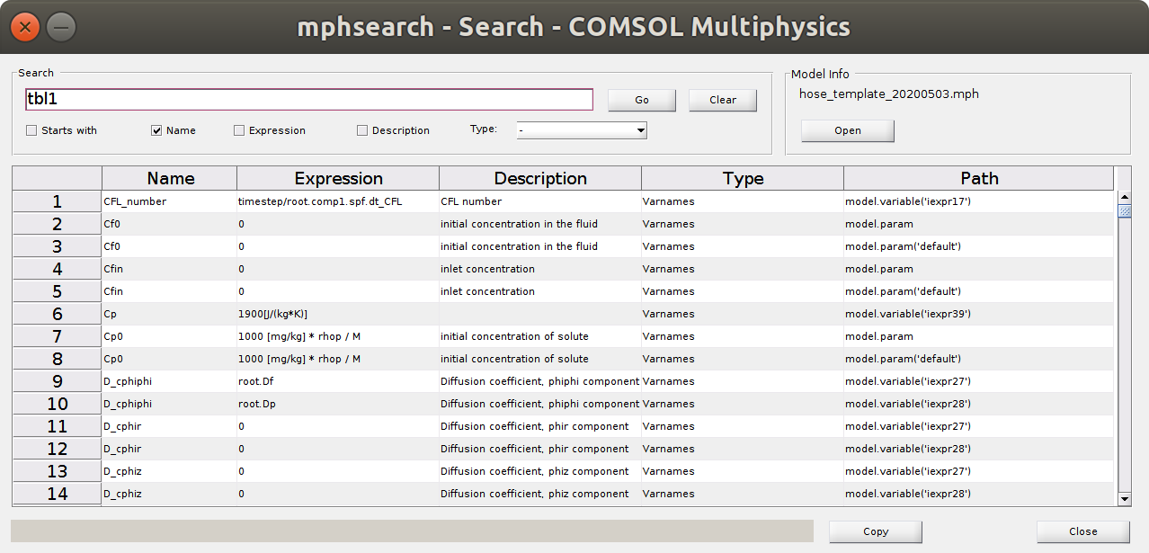
The search engine enables to identify the path and properties of any quantity. The depicted object tbl1 contains the data of the probe1 (Jmig).
figure, mphgeom(model)
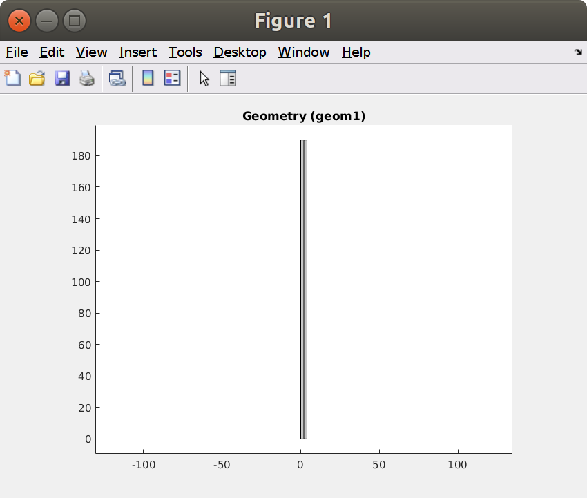
Note that the inlet is in top position () and the outlet at the bottom ().
params = mphgetexpressions(model.param)
params =
14×5 cell array
xxxxxxxxxx{'ri' } {'2 [mm]' } {'internal radius' } {[ 0.0020]} {'m' }{'re' } {'4 [mm]' } {'external radius' } {[ 0.0040]} {'m' }{'L' } {'19 [cm]' } {'hose length' } {[ 0.1900]} {'m' }{'muF' } {'0.04 [Pa*s]' } {'viscosity F (Pa…'} {[ 0.0400]} {'Pa*s' }{'Q' } {'10 [ml/min]' } {'flow rate' } {[1.6667e-07]} {'m^3/s' }{'Patm'} {'100 [kPa]' } {'Atmospheric pre…'} {[ 100000]} {'Pa' }{'Dp' } {'1E-12 [m^2/s]' } {'diffusivity in …'} {[1.0000e-12]} {'m^2/s' }{'Df' } {'1e-9 [m^2/s]' } {'diffusivity in …'} {[1.0000e-09]} {'m^2/s' }{'Kfp' } {'0.001' } {'partition coeff…'} {[1.0000e-03]} {0×0 char }{'rhop'} {'900 [kg/m^3]' } {'hose (P) density' } {[ 900]} {'kg/m^3' }{'M' } {'300 [g/mol]' } {'molecular mass …'} {[ 0.3000]} {'kg/mol' }{'Cp0' } {'1000 [mg/kg] * …'} {'initial concent…'} {[ 3]} {'mol/m^3'}{'Cf0' } {'0' } {'initial concent…'} {[ 0]} {0×0 char }{'Cfin'} {'0' } {'inlet concentra…'} {[ 0]} {0×0 char }`15.3 Global parameters
We need to extract the main parameters of the model to interpret the simulation results.
xxxxxxxxxx%% global parametersL = mphglobal(model,'L'); % do not use mphevaluate(model, 'L'), it does not have the right unitsri = mphglobal(model, 'ri');re = mphglobal(model, 're');% assuming that the geometry is geom1lunit = char(model.component('comp1').geom('geom1').lengthUnit); % length unit as used in the projectlfactor = struct('m',1,'cm',1e-2,'mm',1e-3);lscale = lfactor.(lunit);% assuming that the transport study is std2tlist = model.study('std2').feature('time').getDoubleArray('tlist'); % list of timestunit = char(model.study('std2').feature('time').getString('tunit')); % time unit as used in the projecttfactor = struct('s',1,'min',60); % enter other scales if neededtscale = tfactor.(tunit); tmax = tlist(end);% R0: initial (residual) amount in the materialC0 = mphglobal(model,'Cp0')*mphglobal(model,'M'); % concentration in the material in kg/m3R0 = C0 * pi*(re^2-ri^2)*L * lscale^3; % in kg15.4 Extract concentration profiles along the hose
Concentrations profiles along the hose between (inlet) and (outlet) with a step equal to and 20 time steps chosen on square-root time scale.
xxxxxxxxxx%% coarse method to get profiles for prescribed times and vertical position% we use: model.result('pg10').feature('lngr1')pg = model.result('pg10'); % plot groupcln1 = model.result.dataset('cln1'); % cutting linecln1.label('customized');pg.feature('lngr1').set('expr', 'tds.cmass_c');pg.set('ylabel', 'Mass concentration (kg/m<sup>3</sup>)');pg.set('interp', sprintf('{%s}',sprintf('%d ',round(linspace(0,sqrt(tmax),20)'.^2))));pg.set('data', 'cln1');% change the values herefigureposz = L*(1:-.1:0);for i=1:length(posz) subplot(3,4,i), hold on cln1.set('genpoints', [0 posz(i); re posz(i)]); mphplot(model,'pg10','rangenum',1) title(sprintf('z=%0.3g (%s)',posz(i),lunit))end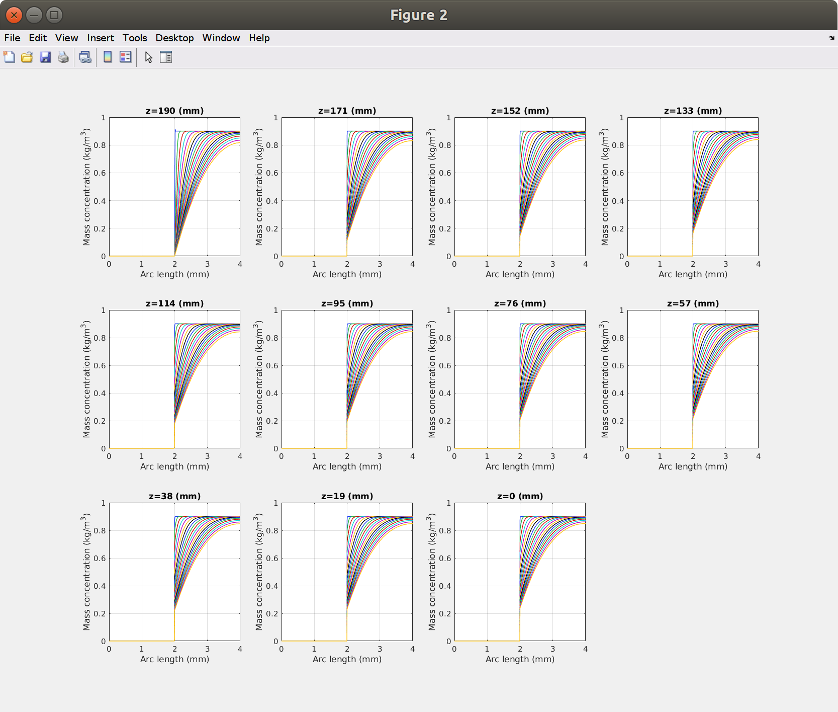
The layout is defined by mphplot().
15.5 Mass balance for probe1: integration of Jmig with time
Comsol calculates surface integrals more accurately than Matlab can do as it as access to the original mesh. It is, however, much easier to carry out post-processing calculations directly in Matlab. The code below calculates the total amount of solute, which has left the hose through the outlet.
xxxxxxxxxx%% Mass balance from the probe (i.e. from the flow)% time samplingnt = 200;t = linspace(0,sqrt(tmax),nt).^2;% Retrieve the data of the probeJmigraw = mpheval(model,'Jmig');Jmig = mphtable(model,'tbl1'); % created with: model.component("comp1").probe("bnd1").set("table", "tbl1");Jmig.unit = Jmigraw.unit{1};Jmig.t = t;Jmig.M = tscale*interp1(Jmig.data(:,1),cumtrapz(Jmig.data(:,1),Jmig.data(:,2)),t,'pchip');Jmig.Munit = 'kg';figure, plot(Jmig.t,Jmig.M,'linewidth',3);xlabel(sprintf('time (%s)',tunit),'fontsize',16)ylabel(sprintf('Total Amount of solute transferred (%s)',Jmig.Munit),'fontsize',16)title('integratral of probe1: \bfJmig with time','fontsize',16)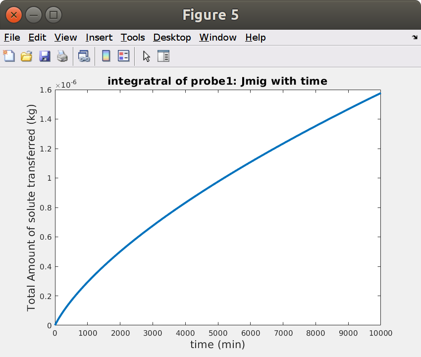
15.6 Mass balance from 2D concentration profiles
The 2D concentration profiles in inner and hose are interpolated on a regular grid. Successive integrations are applied to carry out a full mass balance.
Note that the calculations and the comparison with Jmig.M neglects the amount of solute in inner.
Data interpolation and identification of ROIs (regions of interest)
xxxxxxxxxx%% Mass balance from the residual concentration in the hose% space sampling and unform gridnri = 40;nre = 200;nr = nri+nre;nz = 300;r = [linspace(0,ri-sqrt(eps),nri),linspace(ri+sqrt(eps),re,nre)]; % note two positions across the F-P interfaces separated by sqrt(eps)z = linspace(0,L,nz);[R,Z] = meshgrid(r,z);% identifiation of regions of interest (hose and inner)isinner = (r<ri); ishose = (~isinner);inner = find(isinner); hose = find(ishose);inlet = find(z==L);outlet = find(z==0);middle = find((z>L/3) & (z<2*L/3));% interpmaximum mass balance error (flow vs residual) 1.79% (theoretical: -0.00543%)olation and reshapecmassraw = mpheval(model,'tds.cmass_c');Cunit = cmassraw.unit{1};Cscale = lscale^3;raw = mphinterp(model,'tds.cmass_c','data','dset2','coord',[R(:) Z(:)]','t',t); % t and r x zC = permute(reshape(raw,[nt,nz,nr]),[3 2 1]) * Cscale; % r, z and time% mass balance: Rz: residual amount per length unit along z% total amount: Rz0*LRz = squeeze(trapz(r(hose),C(hose,:,:)*2*pi.*r(hose)',1)); % z and time[TT,ZZ] = meshgrid(t,z);Rz0 = mean(Rz(middle,1)); % initial mass per length unit(estimated from the middle section at t=0)Mz = Rz0 - Rz; % cumulated amount transferred (per length unit) at each z and tM = trapz(z,Mz); % cumulated amount transferred at tMinf = Rz0*L; % maximum amount transferrable (it should be equal to R0)fprintf(1,'maximum mass balance error (flow vs residual) %0.3g%% (theoretical: %0.3g%%)\n',100*(1-Jmig.M(end)/M(end)),100*(1-R0/Minf))>>
maximum mass balance error (flow vs residual) 1.79% (theoretical: -0.00543%)
Plot 2D concentration profiles at prescribed times
xxxxxxxxxx% concentration profileit = 100; %iteration numberfigure, surf(R,Z,C(:,:,100)','edgecolor','none')xlabel(sprintf('r (%s)',lunit),'fontsize',16)ylabel(sprintf('z (%s)',lunit),'fontsize',16)zlabel(sprintf('concentration (%s)',Cunit),'fontsize',16)title(sprintf('2D concentration profile at t=%0.3g %s',t(it),tunit),'fontsize',16)figure, surf(R,Z,C(:,:,it)','edgecolor','none')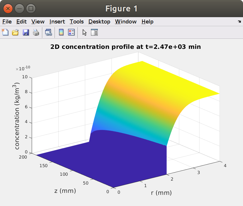
Iso-migration contours vs and
It is obvious that the effects of radii ( and ) cannot be extrapolated from one single simulation. By contrast, the effect of and can be easily extrapolated from a sufficiently long hose and sufficiently long simulations. This feature is shown as iso-migration contours with (contact time) and (length).
Note that the vertical coordinate has been replaced by to get the inlet at the position . The following figure describes the relative loss of solute for each section according to its position respectively to the inlet.
xxxxxxxxxx%% Iso-migration contours *vs* $t$ and $z$figure[cc,hh] = contourf(L-ZZ,TT,Mz./Rz0,.01:.01:.9);clabel(cc,hh)xlabel(sprintf('hose position (%s) - direction of the flow \\bf\\rightarrow',lunit),'fontsize',16)ylabel(sprintf('time (%s)',tunit),'fontsize',16)title('amount transferred for each section')
15.7 Comparison of mass balances (flow and residual amounts)
Note that the amount of solute in the fluid (in inlet) is neglected at each time. As a result, the red curve (from residual concentration) is above the blue one (from the flow leaving through the outlet).
xxxxxxxxxx% Comparison of mass balancesfigure,hp = plot(Jmig.t,Jmig.M/R0,t,M/Minf,'linewidth',3);xlabel(sprintf('time (%s)',tunit),'fontsize',16)ylabel(sprintf('Relative amount of solute transferred (%s)',Jmig.Munit),'fontsize',16)title('Comparison of mass balances','fontsize',16)legend(hp,{'from flow','from residual conc.'},'location','best','fontsize',14,'box','off')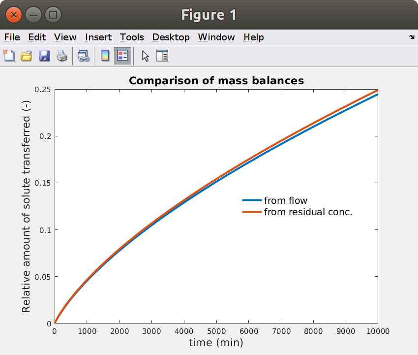
15.8 Launching calculations for different flow rates:
Use the following script as a template to study other effects. Execution time can be beyond 10 min, adjust the number of flow rates before launching it.
Changing the flow rate requires to restart std1.
xxxxxxxxxx%% Comparison of results for different flow rates: Q% use this script as a template to perform sensitivity analysisQ = [0.1 .5 1 5 10 50 100]; % mL/minnQ = length(Q);Qtxt = arrayfun(@(q) sprintf('%0.3g [ml/min]',q),Q,'UniformOutput',false);Qleg = arrayfun(@(q) sprintf('%0.3g ml\\cdotmin^{-1}',q),Q,'UniformOutput',false);figure, hold oncol = parula(nQ); hp =zeros(nQ,1);for i=1:nQ model.param.set('Q', Qtxt{i}, 'flow rate'); model.study("std1").run(); model.study("std2").run(); Jmig = mphtable(model,'tbl1'); % created with: model.component("comp1").probe("bnd1").set("table", "tbl1"); Jmig.unit = Jmigraw.unit{1}; Jmig.t = t; Jmig.M = tscale*interp1(Jmig.data(:,1),cumtrapz(Jmig.data(:,1),Jmig.data(:,2)),t,'pchip'); Jmig.Munit = 'kg'; hp(i) = plot(Jmig.t,Jmig.M,'linewidth',3,'color',col(i,:));endxlabel(sprintf('time (%s)',tunit),'fontsize',16)ylabel(sprintf('Total Amount of solute transferred (%s)',Jmig.Munit),'fontsize',16)title('Effect of flow rate','fontsize',16)legend(hp,Qleg,'location','best','fontsize',14,'box','off')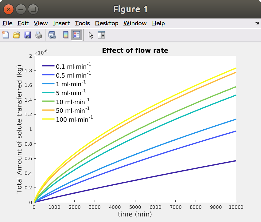
The results confirm previous analysis, increasing flow rate (for a same hose) reduces the effect of (solubility is limiting in these simulations). Simulations evolve from a linear shape (low values) to the typical kinetics vs the square-root of time (high values). The upper limit is a kinetics in a closed system for (Dirichlet condition forcing the concentration to be 0 at the interface). The linear shape can be obtained in closed-systems with low mass Biot numbers ( with ) .
16. THIS TEMPLATE AS A MATLAB FUNCTION
This template is provided for convenience as a Matlab function
xxxxxxxxxxfunction out = model%% hose_template_20200504.m%% Model exported on May 4 2020, 11:17 by COMSOL 5.5.0.359.% INRAe\Olivier Vitrac - rev. 2020-05-04import com.comsol.model.*import com.comsol.model.util.*model = ModelUtil.create('Model');model.modelPath('/home/olivi/Documents/hose');model.label('hose_template_20200503.mph');model.param.set('ri', '2 [mm]', 'internal radius');model.param.set('re', '4 [mm]', 'external radius');model.param.set('L', '19 [cm]', 'hose length');model.param.set('muF', '0.04 [Pa*s]', 'viscosity F (Pa.s)');model.param.set('Q', '10 [ml/min]', 'flow rate');model.param.set('Patm', '100 [kPa]', 'Atmospheric pressure (outlet)');model.param.set('Dp', '1E-12 [m^2/s]', 'diffusivity in the hose (P)');model.param.set('Df', '1e-9 [m^2/s]', 'diffusivity in the fluid (F)');model.param.set('Kfp', '0.001', 'partition coefficient between F and P');model.param.set('rhop', '900 [kg/m^3]', 'hose (P) density');model.param.set('M', '300 [g/mol]', 'molecular mass of solute');model.param.set('Cp0', '1000 [mg/kg] * rhop / M', 'initial concentration of solute');model.param.set('Cf0', '0', 'initial concentration in the fluid');model.param.set('Cfin', '0', 'inlet concentration');model.component.create('comp1', true);model.component('comp1').geom.create('geom1', 2);model.result.table.create('tbl1', 'Table');model.component('comp1').geom('geom1').axisymmetric(true);model.component('comp1').mesh.create('mesh1');model.component('comp1').geom('geom1').lengthUnit('mm');model.component('comp1').geom('geom1').create('r1', 'Rectangle');model.component('comp1').geom('geom1').feature('r1').label('inner');model.component('comp1').geom('geom1').feature('r1').set('size', {'ri' 'L'});model.component('comp1').geom('geom1').create('r2', 'Rectangle');model.component('comp1').geom('geom1').feature('r2').label('hose');model.component('comp1').geom('geom1').feature('r2').set('pos', {'ri' '0'});model.component('comp1').geom('geom1').feature('r2').set('size', {'re-ri' 'L'});model.component('comp1').geom('geom1').run;model.component('comp1').variable.create('var1');model.component('comp1').variable('var1').set('Jmigz', 'linproj1(-tds.tflux_cz*M)', 'J profile along z');model.view.create('view2', 3);model.view.create('view3', 3);model.component('comp1').material.create('mat1', 'Common');model.component('comp1').material.create('mat2', 'Common');model.component('comp1').material('mat1').selection.set([1]);model.component('comp1').material('mat1').propertyGroup('def').func.create('k', 'Piecewise');model.component('comp1').material('mat1').propertyGroup('def').func.create('rho', 'Piecewise');model.component('comp1').material('mat1').propertyGroup('def').func.create('SurfF', 'Piecewise');model.component('comp1').material('mat2').selection.set([2]);model.component('comp1').material('mat2').propertyGroup.create('Enu', 'Young''s modulus and Poisson''s ratio');model.component('comp1').cpl.create('linproj1', 'LinearProjection');model.component('comp1').cpl('linproj1').selection.set([1]);model.component('comp1').physics.create('spf', 'LaminarFlow', 'geom1');model.component('comp1').physics('spf').selection.set([1]);model.component('comp1').physics('spf').create('inl1', 'InletBoundary', 1);model.component('comp1').physics('spf').feature('inl1').selection.set([3]);model.component('comp1').physics('spf').create('out1', 'OutletBoundary', 1);model.component('comp1').physics('spf').feature('out1').selection.set([2]);model.component('comp1').physics.create('tds', 'DilutedSpecies', 'geom1');model.component('comp1').physics('tds').create('cdm2', 'ConvectionDiffusionMigration', 2);model.component('comp1').physics('tds').feature('cdm2').selection.set([2]);model.component('comp1').physics('tds').create('pac1', 'PartitionCondition', 1);model.component('comp1').physics('tds').feature('pac1').selection.set([4]);model.component('comp1').physics('tds').create('in1', 'Inflow', 1);model.component('comp1').physics('tds').feature('in1').selection.set([3]);model.component('comp1').physics('tds').create('out1', 'Outflow', 1);model.component('comp1').physics('tds').feature('out1').selection.set([2]);model.component('comp1').physics('tds').create('init2', 'init', 2);model.component('comp1').physics('tds').feature('init2').selection.set([2]);model.component('comp1').physics('tds').create('mbc1', 'MassBasedConcentrations', 2);model.component('comp1').mesh('mesh1').create('map1', 'Map');model.component('comp1').mesh('mesh1').create('map2', 'Map');model.component('comp1').mesh('mesh1').feature('map1').selection.geom('geom1', 2);model.component('comp1').mesh('mesh1').feature('map1').selection.set([1]);model.component('comp1').mesh('mesh1').feature('map1').create('dis1', 'Distribution');model.component('comp1').mesh('mesh1').feature('map1').create('dis2', 'Distribution');model.component('comp1').mesh('mesh1').feature('map1').feature('dis1').selection.set([2 3]);model.component('comp1').mesh('mesh1').feature('map1').feature('dis2').selection.set([1 4]);model.component('comp1').mesh('mesh1').feature('map2').selection.geom('geom1', 2);model.component('comp1').mesh('mesh1').feature('map2').selection.set([2]);model.component('comp1').mesh('mesh1').feature('map2').create('dis1', 'Distribution');model.component('comp1').mesh('mesh1').feature('map2').create('dis2', 'Distribution');model.component('comp1').mesh('mesh1').feature('map2').feature('dis1').selection.set([5 6]);model.component('comp1').mesh('mesh1').feature('map2').feature('dis2').selection.set([4 7]);model.component('comp1').probe.create('bnd1', 'Boundary');model.component('comp1').probe('bnd1').selection.set([2]);model.result.table('tbl1').label('Probe Table 1');model.component('comp1').view('view1').axis.set('xmin', -97.624755859375);model.component('comp1').view('view1').axis.set('xmax', 101.624755859375);model.component('comp1').view('view1').axis.set('ymin', -9.500007629394531);model.component('comp1').view('view1').axis.set('ymax', 199.5);model.component('comp1').material('mat1').label('Food simulant');model.component('comp1').material('mat1').propertyGroup('def').func('k').set('arg', 'T');model.component('comp1').material('mat1').propertyGroup('def').func('k').set('pieces', {'293.0' '408.0' '0.16'});model.component('comp1').material('mat1').propertyGroup('def').func('rho').label('Piecewise 1');model.component('comp1').material('mat1').propertyGroup('def').func('rho').set('arg', 'T');model.component('comp1').material('mat1').propertyGroup('def').func('rho').set('pieces', {'293.0' '303.0' '920.0'});model.component('comp1').material('mat1').propertyGroup('def').func('SurfF').label('Piecewise 2');model.component('comp1').material('mat1').propertyGroup('def').func('SurfF').set('arg', 'T');model.component('comp1').material('mat1').propertyGroup('def').func('SurfF').set('pieces', {'293.0' '493.0' '0.04601241-4.761868E-5*T^1'});model.component('comp1').material('mat1').propertyGroup('def').set('thermalconductivity', {'k(T[1/K])[W/(m*K)]' '0' '0' '0' 'k(T[1/K])[W/(m*K)]' '0' '0' '0' 'k(T[1/K])[W/(m*K)]'});model.component('comp1').material('mat1').propertyGroup('def').set('thermalconductivity_symmetry', '0');model.component('comp1').material('mat1').propertyGroup('def').set('density', 'rho(T[1/K])[kg/m^3]');model.component('comp1').material('mat1').propertyGroup('def').set('SurfF', 'SurfF(T[1/K])[N/m]');model.component('comp1').material('mat1').propertyGroup('def').set('dynamicviscosity', 'muF');model.component('comp1').material('mat1').propertyGroup('def').addInput('temperature');model.component('comp1').material('mat2').label('Polyethylene');model.component('comp1').material('mat2').propertyGroup('def').set('thermalexpansioncoefficient', {'150e-6[1/K]' '0' '0' '0' '150e-6[1/K]' '0' '0' '0' '150e-6[1/K]'});model.component('comp1').material('mat2').propertyGroup('def').descr('thermalexpansioncoefficient_symmetry', '');model.component('comp1').material('mat2').propertyGroup('def').set('heatcapacity', '1900[J/(kg*K)]');model.component('comp1').material('mat2').propertyGroup('def').descr('heatcapacity_symmetry', '');model.component('comp1').material('mat2').propertyGroup('def').set('relpermittivity', {'2.3' '0' '0' '0' '2.3' '0' '0' '0' '2.3'});model.component('comp1').material('mat2').propertyGroup('def').descr('relpermittivity_symmetry', '');model.component('comp1').material('mat2').propertyGroup('def').set('density', '930[kg/m^3]');model.component('comp1').material('mat2').propertyGroup('def').descr('density_symmetry', '');model.component('comp1').material('mat2').propertyGroup('def').set('thermalconductivity', {'0.38[W/(m*K)]' '0' '0' '0' '0.38[W/(m*K)]' '0' '0' '0' '0.38[W/(m*K)]'});model.component('comp1').material('mat2').propertyGroup('def').descr('thermalconductivity_symmetry', '');model.component('comp1').material('mat2').propertyGroup('Enu').set('youngsmodulus', '1e9[Pa]');model.component('comp1').material('mat2').propertyGroup('Enu').descr('youngsmodulus_symmetry', '');model.component('comp1').material('mat2').propertyGroup('Enu').descr('poissonsratio_symmetry', '');model.component('comp1').cpl('linproj1').selection('srcvertex1').set([2]);model.component('comp1').cpl('linproj1').selection('srcvertex2').set([4]);model.component('comp1').cpl('linproj1').selection('srcvertex3').set([3]);model.component('comp1').cpl('linproj1').selection('dstvertex1').set([2]);model.component('comp1').cpl('linproj1').selection('dstvertex2').set([1]);model.component('comp1').physics('spf').prop('PhysicalModelProperty').set('Compressibility', 'WeaklyCompressible');model.component('comp1').physics('spf').prop('PhysicalModelProperty').set('Tref', '313.15[K]');model.component('comp1').physics('spf').feature('inl1').set('BoundaryCondition', 'FullyDevelopedFlow');model.component('comp1').physics('spf').feature('inl1').set('FullyDevelopedFlowOption', 'V0');model.component('comp1').physics('spf').feature('inl1').set('V0fdf', 'Q');model.component('comp1').physics('spf').feature('out1').set('p0', 'Patm');model.component('comp1').physics('tds').prop('EquationForm').set('form', 'Transient');model.component('comp1').physics('tds').feature('cdm1').set('u_src', 'root.comp1.u');model.component('comp1').physics('tds').feature('cdm1').set('D_c', {'Df'; '0'; '0'; '0'; 'Df'; '0'; '0'; '0'; 'Df'});model.component('comp1').physics('tds').feature('init1').set('initc', 'Cf0');model.component('comp1').physics('tds').feature('cdm2').set('D_c', {'Dp'; '0'; '0'; '0'; 'Dp'; '0'; '0'; '0'; 'Dp'});model.component('comp1').physics('tds').feature('pac1').set('ReverseDirection', true);model.component('comp1').physics('tds').feature('pac1').set('K', 'Kfp');model.component('comp1').physics('tds').feature('in1').set('c0', 'Cfin');model.component('comp1').physics('tds').feature('init2').set('initc', 'Cp0');model.component('comp1').physics('tds').feature('mbc1').set('M_c', 'M');model.component('comp1').mesh('mesh1').feature('map1').feature('dis1').set('type', 'predefined');model.component('comp1').mesh('mesh1').feature('map1').feature('dis1').set('elemcount', 20);model.component('comp1').mesh('mesh1').feature('map1').feature('dis1').set('elemratio', 25);model.component('comp1').mesh('mesh1').feature('map1').feature('dis2').set('numelem', 50);model.component('comp1').mesh('mesh1').feature('map2').feature('dis1').set('type', 'predefined');model.component('comp1').mesh('mesh1').feature('map2').feature('dis1').set('reverse', true);model.component('comp1').mesh('mesh1').feature('map2').feature('dis1').set('elemcount', 30);model.component('comp1').mesh('mesh1').feature('map2').feature('dis1').set('elemratio', 25);model.component('comp1').mesh('mesh1').feature('map2').feature('dis2').set('numelem', 50);model.component('comp1').mesh('mesh1').run;model.component('comp1').probe('bnd1').label('migration rate');model.component('comp1').probe('bnd1').set('type', 'integral');model.component('comp1').probe('bnd1').set('probename', 'Jmig');model.component('comp1').probe('bnd1').set('expr', '-tds.tflux_cz*M');model.component('comp1').probe('bnd1').set('unit', 'kg/s');model.component('comp1').probe('bnd1').set('descr', '-tds.tflux_cz*M');model.component('comp1').probe('bnd1').set('intsurface', true);model.component('comp1').probe('bnd1').set('table', 'tbl1');model.component('comp1').probe('bnd1').set('window', 'window1');model.study.create('std1');model.study('std1').create('stat', 'Stationary');model.study('std1').feature('stat').set('activate', {'spf' 'on' 'tds' 'off' 'frame:spatial1' 'on' 'frame:material1' 'on'});model.study.create('std2');model.study('std2').create('time', 'Transient');model.sol.create('sol1');model.sol('sol1').study('std1');model.sol('sol1').attach('std1');model.sol('sol1').create('st1', 'StudyStep');model.sol('sol1').create('v1', 'Variables');model.sol('sol1').create('s1', 'Stationary');model.sol('sol1').feature('s1').create('fc1', 'FullyCoupled');model.sol('sol1').feature('s1').create('d1', 'Direct');model.sol('sol1').feature('s1').create('i1', 'Iterative');model.sol('sol1').feature('s1').feature('i1').create('mg1', 'Multigrid');model.sol('sol1').feature('s1').feature('i1').feature('mg1').feature('pr').create('sc1', 'SCGS');model.sol('sol1').feature('s1').feature('i1').feature('mg1').feature('po').create('sc1', 'SCGS');model.sol('sol1').feature('s1').feature('i1').feature('mg1').feature('cs').create('d1', 'Direct');model.sol('sol1').feature('s1').feature.remove('fcDef');model.sol.create('sol2');model.sol('sol2').study('std2');model.sol('sol2').attach('std2');model.sol('sol2').create('st1', 'StudyStep');model.sol('sol2').create('v1', 'Variables');model.sol('sol2').create('t1', 'Time');model.sol('sol2').feature('t1').create('fc1', 'FullyCoupled');model.sol('sol2').feature('t1').create('d1', 'Direct');model.sol('sol2').feature('t1').create('i1', 'Iterative');model.sol('sol2').feature('t1').feature('i1').create('mg1', 'Multigrid');model.sol('sol2').feature('t1').feature('i1').feature('mg1').feature('pr').create('sc1', 'SCGS');model.sol('sol2').feature('t1').feature('i1').feature('mg1').feature('po').create('sc1', 'SCGS');model.sol('sol2').feature('t1').feature('i1').feature('mg1').feature('cs').create('d1', 'Direct');model.sol('sol2').feature('t1').feature.remove('fcDef');model.result.dataset.create('rev1', 'Revolve2D');model.result.dataset.create('rev2', 'Revolve2D');model.result.dataset.create('dset3', 'Solution');model.result.dataset.create('int1', 'Integral');model.result.dataset.create('cln1', 'CutLine2D');model.result.dataset.create('cln2', 'CutLine2D');model.result.dataset.create('cln3', 'CutLine2D');model.result.dataset.create('cln4', 'CutLine2D');model.result.dataset('rev2').set('data', 'dset2');model.result.dataset('dset3').set('probetag', 'bnd1');model.result.dataset('dset3').set('solution', 'sol2');model.result.dataset('int1').set('probetag', 'bnd1');model.result.dataset('int1').set('data', 'dset3');model.result.dataset('int1').selection.geom('geom1', 1);model.result.dataset('int1').selection.set([2]);model.result.dataset('cln1').set('data', 'dset2');model.result.dataset('cln2').set('data', 'dset2');model.result.dataset('cln3').set('data', 'dset2');model.result.dataset('cln4').set('data', 'dset2');model.result.numerical.create('pev1', 'EvalPoint');model.result.numerical('pev1').set('probetag', 'bnd1');model.result.create('pg1', 'PlotGroup2D');model.result.create('pg2', 'PlotGroup2D');model.result.create('pg3', 'PlotGroup3D');model.result.create('pg4', 'PlotGroup2D');model.result.create('pg5', 'PlotGroup2D');model.result.create('pg6', 'PlotGroup3D');model.result.create('pg7', 'PlotGroup2D');model.result.create('pg8', 'PlotGroup3D');model.result.create('pg9', 'PlotGroup1D');model.result.create('pg10', 'PlotGroup1D');model.result.create('pg11', 'PlotGroup1D');model.result.create('pg12', 'PlotGroup1D');model.result.create('pg13', 'PlotGroup1D');model.result.create('pg14', 'PlotGroup1D');model.result('pg1').create('surf1', 'Surface');model.result('pg2').create('con1', 'Contour');model.result('pg2').feature('con1').set('expr', 'p');model.result('pg3').create('surf1', 'Surface');model.result('pg4').set('data', 'dset2');model.result('pg4').create('surf1', 'Surface');model.result('pg5').set('data', 'dset2');model.result('pg5').create('con1', 'Contour');model.result('pg5').feature('con1').set('expr', 'p');model.result('pg6').create('surf1', 'Surface');model.result('pg7').set('data', 'dset2');model.result('pg7').create('surf1', 'Surface');model.result('pg7').create('str1', 'Streamline');model.result('pg7').feature('surf1').set('expr', 'c');model.result('pg8').create('surf1', 'Surface');model.result('pg8').feature('surf1').set('expr', 'c');model.result('pg9').set('probetag', 'window1_default');model.result('pg9').create('tblp1', 'Table');model.result('pg9').feature('tblp1').set('probetag', 'bnd1');model.result('pg10').create('lngr1', 'LineGraph');model.result('pg10').feature('lngr1').set('expr', 'tds.cmass_c');model.result('pg11').create('lngr1', 'LineGraph');model.result('pg11').feature('lngr1').set('expr', 'tds.cmass_c');model.result('pg12').create('lngr1', 'LineGraph');model.result('pg12').feature('lngr1').set('expr', 'Jmig');model.result('pg13').create('lngr1', 'LineGraph');model.result('pg13').feature('lngr1').set('expr', 'tds.cmass_c');model.result('pg14').create('lngr1', 'LineGraph');model.result('pg14').feature('lngr1').set('xdata', 'reversedarc');model.result('pg14').feature('lngr1').selection.set([2]);model.component('comp1').probe('bnd1').genResult([]);model.study('std2').feature('time').set('tunit', 'min');model.study('std2').feature('time').set('tlist', '({range(0,0.05,sqrt(10000))})^2');model.study('std2').feature('time').set('usertol', true);model.study('std2').feature('time').set('rtol', '0.0001');model.sol('sol1').attach('std1');model.sol('sol1').feature('s1').feature('aDef').set('cachepattern', true);model.sol('sol1').feature('s1').feature('fc1').set('linsolver', 'd1');model.sol('sol1').feature('s1').feature('fc1').set('initstep', 0.01);model.sol('sol1').feature('s1').feature('fc1').set('maxiter', 100);model.sol('sol1').feature('s1').feature('d1').label('Direct, fluid flow variables (spf)');model.sol('sol1').feature('s1').feature('d1').set('linsolver', 'pardiso');model.sol('sol1').feature('s1').feature('d1').set('pivotperturb', 1.0E-13);model.sol('sol1').feature('s1').feature('i1').label('AMG, fluid flow variables (spf)');model.sol('sol1').feature('s1').feature('i1').set('nlinnormuse', true);model.sol('sol1').feature('s1').feature('i1').set('maxlinit', 200);model.sol('sol1').feature('s1').feature('i1').set('rhob', 20);model.sol('sol1').feature('s1').feature('i1').feature('mg1').set('prefun', 'saamg');model.sol('sol1').feature('s1').feature('i1').feature('mg1').set('maxcoarsedof', 80000);model.sol('sol1').feature('s1').feature('i1').feature('mg1').set('strconn', 0.02);model.sol('sol1').feature('s1').feature('i1').feature('mg1').set('saamgcompwise', true);model.sol('sol1').feature('s1').feature('i1').feature('mg1').set('usesmooth', false);model.sol('sol1').feature('s1').feature('i1').feature('mg1').feature('pr').feature('sc1').set('linesweeptype', 'ssor');model.sol('sol1').feature('s1').feature('i1').feature('mg1').feature('pr').feature('sc1').set('iter', 0);model.sol('sol1').feature('s1').feature('i1').feature('mg1').feature('pr').feature('sc1').set('scgsvertexrelax', 0.7);model.sol('sol1').feature('s1').feature('i1').feature('mg1').feature('pr').feature('sc1').set('vankavarsactive', true);model.sol('sol1').feature('s1').feature('i1').feature('mg1').feature('pr').feature('sc1').set('vankavars', {'comp1_spf_inl1_Pinlfdf'});model.sol('sol1').feature('s1').feature('i1').feature('mg1').feature('po').feature('sc1').set('linesweeptype', 'ssor');model.sol('sol1').feature('s1').feature('i1').feature('mg1').feature('po').feature('sc1').set('iter', 1);model.sol('sol1').feature('s1').feature('i1').feature('mg1').feature('po').feature('sc1').set('scgsvertexrelax', 0.7);model.sol('sol1').feature('s1').feature('i1').feature('mg1').feature('po').feature('sc1').set('vankavarsactive', true);model.sol('sol1').feature('s1').feature('i1').feature('mg1').feature('po').feature('sc1').set('vankavars', {'comp1_spf_inl1_Pinlfdf'});model.sol('sol1').feature('s1').feature('i1').feature('mg1').feature('cs').feature('d1').set('linsolver', 'pardiso');model.sol('sol1').feature('s1').feature('i1').feature('mg1').feature('cs').feature('d1').set('pivotperturb', 1.0E-13);model.sol('sol1').runAll;model.sol('sol2').attach('std2');model.sol('sol2').feature('v1').set('clist', {'({range(0,0.05,sqrt(10000))})^2' '10.0[min]'});model.sol('sol2').feature('t1').set('tunit', 'min');model.sol('sol2').feature('t1').set('tlist', '({range(0,0.05,sqrt(10000))})^2');model.sol('sol2').feature('t1').set('rtol', '0.0001');model.sol('sol2').feature('t1').set('atolglobalfactor', 0.05);model.sol('sol2').feature('t1').set('atolmethod', {'comp1_c' 'global' 'comp1_p' 'scaled' 'comp1_u' 'global' 'comp1_spf_inl1_Pinlfdf' 'global'});model.sol('sol2').feature('t1').set('atolfactor', {'comp1_c' '0.1' 'comp1_p' '1' 'comp1_u' '0.1' 'comp1_spf_inl1_Pinlfdf' '0.1'});model.sol('sol2').feature('t1').set('maxorder', 2);model.sol('sol2').feature('t1').set('stabcntrl', true);model.sol('sol2').feature('t1').set('bwinitstepfrac', 0.01);model.sol('sol2').feature('t1').set('estrat', 'exclude');model.sol('sol2').feature('t1').feature('aDef').set('cachepattern', true);model.sol('sol2').feature('t1').feature('fc1').set('linsolver', 'd1');model.sol('sol2').feature('t1').feature('fc1').set('maxiter', 8);model.sol('sol2').feature('t1').feature('fc1').set('ntolfact', 0.5);model.sol('sol2').feature('t1').feature('fc1').set('damp', 0.9);model.sol('sol2').feature('t1').feature('fc1').set('jtech', 'once');model.sol('sol2').feature('t1').feature('fc1').set('stabacc', 'aacc');model.sol('sol2').feature('t1').feature('fc1').set('aaccdim', 5);model.sol('sol2').feature('t1').feature('fc1').set('aaccmix', 0.9);model.sol('sol2').feature('t1').feature('fc1').set('aaccdelay', 1);model.sol('sol2').feature('t1').feature('d1').label('Direct, fluid flow variables (spf) (merged)');model.sol('sol2').feature('t1').feature('d1').set('linsolver', 'pardiso');model.sol('sol2').feature('t1').feature('d1').set('pivotperturb', 1.0E-13);model.sol('sol2').feature('t1').feature('i1').label('AMG, fluid flow variables (spf)');model.sol('sol2').feature('t1').feature('i1').set('maxlinit', 50);model.sol('sol2').feature('t1').feature('i1').set('rhob', 20);model.sol('sol2').feature('t1').feature('i1').feature('mg1').set('prefun', 'saamg');model.sol('sol2').feature('t1').feature('i1').feature('mg1').set('maxcoarsedof', 80000);model.sol('sol2').feature('t1').feature('i1').feature('mg1').set('strconn', 0.02);model.sol('sol2').feature('t1').feature('i1').feature('mg1').set('saamgcompwise', true);model.sol('sol2').feature('t1').feature('i1').feature('mg1').set('usesmooth', false);model.sol('sol2').feature('t1').feature('i1').feature('mg1').feature('pr').feature('sc1').set('linesweeptype', 'ssor');model.sol('sol2').feature('t1').feature('i1').feature('mg1').feature('pr').feature('sc1').set('iter', 0);model.sol('sol2').feature('t1').feature('i1').feature('mg1').feature('pr').feature('sc1').set('scgsvertexrelax', 0.7);model.sol('sol2').feature('t1').feature('i1').feature('mg1').feature('pr').feature('sc1').set('vankavarsactive', true);model.sol('sol2').feature('t1').feature('i1').feature('mg1').feature('pr').feature('sc1').set('vankavars', {'comp1_spf_inl1_Pinlfdf'});model.sol('sol2').feature('t1').feature('i1').feature('mg1').feature('po').feature('sc1').set('linesweeptype', 'ssor');model.sol('sol2').feature('t1').feature('i1').feature('mg1').feature('po').feature('sc1').set('iter', 1);model.sol('sol2').feature('t1').feature('i1').feature('mg1').feature('po').feature('sc1').set('scgsvertexrelax', 0.7);model.sol('sol2').feature('t1').feature('i1').feature('mg1').feature('po').feature('sc1').set('vankavarsactive', true);model.sol('sol2').feature('t1').feature('i1').feature('mg1').feature('po').feature('sc1').set('vankavars', {'comp1_spf_inl1_Pinlfdf'});model.sol('sol2').feature('t1').feature('i1').feature('mg1').feature('cs').feature('d1').set('linsolver', 'pardiso');model.sol('sol2').feature('t1').feature('i1').feature('mg1').feature('cs').feature('d1').set('pivotperturb', 1.0E-13);model.sol('sol2').runAll;model.result.dataset('rev1').label('Revolution 2D');model.result.dataset('rev1').set('startangle', -90);model.result.dataset('rev1').set('revangle', 225);model.result.dataset('rev2').label('Revolution 2D 1');model.result.dataset('rev2').set('startangle', -90);model.result.dataset('rev2').set('revangle', 225);model.result.dataset('dset3').label('Probe Solution 3');model.result.dataset('cln1').label('middle');model.result.dataset('cln1').set('genpoints', {'0' 'L/2'; 'ri+re' 'L/2'});model.result.dataset('cln2').label('outlet');model.result.dataset('cln2').set('genpoints', {'0' '0'; 'ri+re' '0'});model.result.dataset('cln2').set('spacevars', {'cln1x'});model.result.dataset('cln2').set('normal', {'cln1nx' 'cln1ny'});model.result.dataset('cln3').label('axis');model.result.dataset('cln3').set('genpoints', {'0' 'L'; '0' '0'});model.result.dataset('cln3').set('spacevars', {'cln1x'});model.result.dataset('cln3').set('normal', {'cln1nx' 'cln1ny'});model.result.dataset('cln4').label('inlet');model.result.dataset('cln4').set('genpoints', {'0' 'L'; 'ri+re' 'L'});model.result.dataset('cln4').set('spacevars', {'cln1x'});model.result.dataset('cln4').set('normal', {'cln1nx' 'cln1ny'});model.result.create('pg9', 'PlotGroup1D');model.result('pg1').label('Velocity (spf)');model.result('pg1').set('frametype', 'spatial');model.result('pg1').feature('surf1').label('Surface');model.result('pg1').feature('surf1').set('colortable', 'Spectrum');model.result('pg1').feature('surf1').set('smooth', 'internal');model.result('pg1').feature('surf1').set('resolution', 'normal');model.result('pg2').label('Pressure (spf)');model.result('pg2').set('frametype', 'spatial');model.result('pg2').feature('con1').label('Contour');model.result('pg2').feature('con1').set('number', 40);model.result('pg2').feature('con1').set('levelrounding', false);model.result('pg2').feature('con1').set('smooth', 'internal');model.result('pg2').feature('con1').set('resolution', 'normal');model.result('pg3').label('Velocity, 3D (spf)');model.result('pg3').set('frametype', 'spatial');model.result('pg3').feature('surf1').label('Surface');model.result('pg3').feature('surf1').set('smooth', 'internal');model.result('pg3').feature('surf1').set('resolution', 'normal');model.result('pg4').label('Velocity (spf) 1');model.result('pg4').set('frametype', 'spatial');model.result('pg4').feature('surf1').label('Surface');model.result('pg4').feature('surf1').set('smooth', 'internal');model.result('pg4').feature('surf1').set('resolution', 'normal');model.result('pg5').label('Pressure (spf) 1');model.result('pg5').set('frametype', 'spatial');model.result('pg5').feature('con1').label('Contour');model.result('pg5').feature('con1').set('number', 40);model.result('pg5').feature('con1').set('levelrounding', false);model.result('pg5').feature('con1').set('smooth', 'internal');model.result('pg5').feature('con1').set('resolution', 'normal');model.result('pg6').label('Velocity, 3D (spf) 1');model.result('pg6').set('data', 'rev2');model.result('pg6').set('looplevel', [2001]);model.result('pg6').set('frametype', 'spatial');model.result('pg6').feature('surf1').label('Surface');model.result('pg6').feature('surf1').set('smooth', 'internal');model.result('pg6').feature('surf1').set('resolution', 'normal');model.result('pg7').label('Concentration (tds)');model.result('pg7').set('titletype', 'custom');model.result('pg7').feature('surf1').set('resolution', 'normal');model.result('pg7').feature('str1').set('expr', {'tds.tflux_cr' 'tds.tflux_cz'});model.result('pg7').feature('str1').set('descr', 'Total flux');model.result('pg7').feature('str1').set('posmethod', 'uniform');model.result('pg7').feature('str1').set('pointtype', 'arrow');model.result('pg7').feature('str1').set('arrowcount', 7);model.result('pg7').feature('str1').set('arrowlength', 'logarithmic');model.result('pg7').feature('str1').set('arrowscale', 5732968.201703273);model.result('pg7').feature('str1').set('color', 'gray');model.result('pg7').feature('str1').set('recover', 'pprint');model.result('pg7').feature('str1').set('arrowcountactive', false);model.result('pg7').feature('str1').set('arrowscaleactive', false);model.result('pg7').feature('str1').set('resolution', 'normal');model.result('pg8').label('Concentration, 3D (tds)');model.result('pg8').set('data', 'rev2');model.result('pg8').set('looplevel', [2001]);model.result('pg8').set('titletype', 'custom');model.result('pg8').set('typeintitle', false);model.result('pg8').feature('surf1').set('resolution', 'normal');model.result('pg9').label('Probe Plot Group 9');model.result('pg9').set('data', 'none');model.result('pg9').set('xlabel', 'Time (min)');model.result('pg9').set('ylabel', '-tds.tflux_cz*M (kg/s), migration rate');model.result('pg9').set('window', 'window1');model.result('pg9').set('windowtitle', 'Probe Plot 1');model.result('pg9').set('xlabelactive', false);model.result('pg9').set('ylabelactive', false);model.result('pg9').create('tblp1', 'Table');model.result('pg9').feature('tblp1').label('Probe Table Graph 1');model.result('pg9').feature('tblp1').set('plotcolumninput', 'manual');model.result('pg9').feature('tblp1').set('legend', true);model.result('pg10').label('1D middle cross-section');model.result('pg10').set('data', 'cln1');model.result('pg10').set('looplevelinput', {'interp'});model.result('pg10').set('interp', {'range(0,100,10000)'});model.result('pg10').set('xlabel', 'Arc length (mm)');model.result('pg10').set('ylabel', 'Mass concentration (kg/m<sup>3</sup>)');model.result('pg10').set('xlabelactive', false);model.result('pg10').set('ylabelactive', false);model.result('pg10').feature('lngr1').set('resolution', 'normal');model.result('pg11').label('1D outlet cross-section');model.result('pg11').set('data', 'cln2');model.result('pg11').set('looplevelinput', {'interp'});model.result('pg11').set('interp', {'range(0,100,10000)'});model.result('pg11').set('xlabel', 'Arc length (mm)');model.result('pg11').set('ylabel', 'Mass concentration (kg/m<sup>3</sup>)');model.result('pg11').set('xlabelactive', false);model.result('pg11').set('ylabelactive', false);model.result('pg11').feature('lngr1').set('resolution', 'normal');model.result('pg12').label('1D axis profile');model.result('pg12').set('data', 'cln3');model.result('pg12').set('looplevelinput', {'interp'});model.result('pg12').set('interp', {'range(0,100,10000)'});model.result('pg12').set('xlabel', 'Arc length (mm)');model.result('pg12').set('ylabel', 'Probe variable Jmig (kg/s)');model.result('pg12').set('xlabelactive', false);model.result('pg12').set('ylabelactive', false);model.result('pg12').feature('lngr1').set('resolution', 'normal');model.result('pg13').label('1D inlet cross-section 1');model.result('pg13').set('data', 'cln4');model.result('pg13').set('looplevelinput', {'interp'});model.result('pg13').set('interp', {'range(0,100,10000)'});model.result('pg13').set('xlabel', 'Arc length (mm)');model.result('pg13').set('ylabel', 'Mass concentration (kg/m<sup>3</sup>)');model.result('pg13').set('xlabelactive', false);model.result('pg13').set('ylabelactive', false);model.result('pg13').feature('lngr1').set('resolution', 'normal');model.result('pg14').label('1D Velocities');model.result('pg14').set('xlabel', 'Reversed arc length (mm)');model.result('pg14').set('ylabel', 'Velocity magnitude (m/s)');model.result('pg14').set('xlabelactive', false);model.result('pg14').set('ylabelactive', false);model.result('pg14').feature('lngr1').set('resolution', 'normal');model.result.remove('pg15');out = model;17. THE EXAMPLES AS A SINGLE SCRIPT
For convenience, the detailed examples above are given as a single script. Be patient, if you run it at once.
Do not forget to launch Matlab with Comsol as a server.See instructions in 15.1.
xxxxxxxxxx%% EXAMPLES INCLUDED IN THE TEMPLATE: Migration from hoses% INRAe\Olivier Vitrac - rev. 2020-05-05% run Matlab with Comsol as a server% comsol mphserver matlab%% Start a new model from scratchmodel = hose_template_20200504();%% alternatively, load an existing modelmodel = mphopen('hose_template_20200504.mph');%% explore the modelnfo = mphsolutioninfo(model);for s = nfo.solutions' if ~iscellstr(nfo.(s{1}).dataset), nfo.(s{1}).dataset = {nfo.(s{1}).dataset}; end fprintf(1,'Solution ''%s'' with datasets: %s\n',s{1},sprintf('''%s'' ',nfo.(s{1}).dataset{:}));endmphnavigatorfigure, mphgeom(model) % plot the geometry modelparams = mphgetexpressions(model.param) % display all parameters%% global parametersL = mphglobal(model,'L'); % do not use mphevaluate(model, 'L'), it does not have the right unitsri = mphglobal(model, 'ri');re = mphglobal(model, 're');% assuming that the geometry is geom1lunit = char(model.component('comp1').geom('geom1').lengthUnit); % length unit as used in the projectlfactor = struct('m',1,'cm',1e-2,'mm',1e-3);lscale = lfactor.(lunit);% assuming that the transport study is std2tlist = model.study('std2').feature('time').getDoubleArray('tlist'); % list of timestunit = char(model.study('std2').feature('time').getString('tunit')); % time unit as used in the projecttfactor = struct('s',1,'min',60); % enter other scales if neededtscale = tfactor.(tunit); tmax = tlist(end);% R0: initial (residual) amount in the materialC0 = mphglobal(model,'Cp0')*mphglobal(model,'M'); % concentration in the material in kg/m3R0 = C0 * pi*(re^2-ri^2)*L * lscale^3; % in kg%% coarse method to get profiles for prescribed times and vertical position% we use: model.result('pg10').feature('lngr1')pg = model.result('pg10'); % plot groupcln1 = model.result.dataset('cln1'); % cutting linecln1.label('customized');pg.feature('lngr1').set('expr', 'tds.cmass_c');pg.set('ylabel', 'Mass concentration (kg/m<sup>3</sup>)');pg.set('interp', sprintf('{%s}',sprintf('%d ',round(linspace(0,sqrt(tmax),20)'.^2))));pg.set('data', 'cln1');% change the values herefigureposz = L*(1:-.1:0);for i=1:length(posz) subplot(3,4,i), hold on cln1.set('genpoints', [0 posz(i); re posz(i)]); mphplot(model,'pg10','rangenum',1) title(sprintf('z=%0.3g (%s)',posz(i),lunit))end%% Mass balance from the probe (i.e. from the flow)% time samplingnt = 200;t = linspace(0,sqrt(tmax),nt).^2;% Retrieve the data of the probeJmigraw = mpheval(model,'Jmig');Jmig = mphtable(model,'tbl1'); % created with: model.component("comp1").probe("bnd1").set("table", "tbl1");Jmig.unit = Jmigraw.unit{1};Jmig.t = t;Jmig.M = tscale*interp1(Jmig.data(:,1),cumtrapz(Jmig.data(:,1),Jmig.data(:,2)),t,'pchip');Jmig.Munit = 'kg';figure, plot(Jmig.t,Jmig.M,'linewidth',3);xlabel(sprintf('time (%s)',tunit),'fontsize',16)ylabel(sprintf('Total Amount of solute transferred (%s)',Jmig.Munit),'fontsize',16)title('integratral of probe1: \bfJmig with time','fontsize',16)%% Mass balance from the residual concentration in the hose% space sampling and unform gridnri = 40;nre = 200;nr = nri+nre;nz = 300;r = [linspace(0,ri-sqrt(eps),nri),linspace(ri+sqrt(eps),re,nre)]; % note two positions across the F-P interfaces separated by sqrt(eps)z = linspace(0,L,nz);[R,Z] = meshgrid(r,z);% identifiation of regions of interest (hose and inner)isinner = (r<ri); ishose = (~isinner);inner = find(isinner); hose = find(ishose);inlet = find(z==L);outlet = find(z==0);middle = find((z>L/3) & (z<2*L/3));% interpolation and reshapecmassraw = mpheval(model,'tds.cmass_c');Cunit = cmassraw.unit{1};Cscale = lscale^3;raw = mphinterp(model,'tds.cmass_c','data','dset2','coord',[R(:) Z(:)]','t',t); % t and r x zC = permute(reshape(raw,[nt,nz,nr]),[3 2 1]) * Cscale; % r, z and time% mass balance: Rz: residual amount per length unit along z% total amount: Rz0*LRz = squeeze(trapz(r(hose),C(hose,:,:)*2*pi.*r(hose)',1)); % z and time[TT,ZZ] = meshgrid(t,z);Rz0 = mean(Rz(middle,1)); % initial mass per length unit(estimated from the middle section at t=0)Mz = Rz0 - Rz; % cumulated amount transferred (per length unit) at each z and tM = trapz(z,Mz); % cumulated amount transferred at tMinf = Rz0*L; % maximum amount transferrable (it should be equal to R0)fprintf(1,'maximum mass balance error (flow vs residual) %0.3g%% (theoretical: %0.3g%%)\n',100*(1-Jmig.M(end)/M(end)),100*(1-R0/Minf))%% Simple figures% concentration profileit = 100;xlabel(sprintf('r (%s)',lunit),'fontsize',16)ylabel(sprintf('z (%s)',lunit),'fontsize',16)zlabel(sprintf('concentration (%s)',Cunit),'fontsize',16)title(sprintf('2D concentration profile at t=%0.3g %s',t(it),tunit),'fontsize',16)figure, surf(R,Z,C(:,:,it)','edgecolor','none')% Iso-migration contours vs t and zfigure[cc,hh] = contourf(L-ZZ,TT,Mz./Rz0,.01:.01:.9);clabel(cc,hh)xlabel(sprintf('hose position (%s) - direction of the flow \\bf\\rightarrow',lunit),'fontsize',16)ylabel(sprintf('time (%s)',tunit),'fontsize',16)title('amount transferred for each section')% Comparison of mass balancesfigure,hp = plot(Jmig.t,Jmig.M/R0,t,M/Minf,'linewidth',3);xlabel(sprintf('time (%s)',tunit),'fontsize',16)ylabel(sprintf('Relative amount of solute transferred (%s)',Jmig.Munit),'fontsize',16)title('Comparison of mass balances','fontsize',16)legend(hp,{'from flow','from residual conc.'},'location','best','fontsize',14,'box','off')%% Comparison of results for different flow rates: Q% use this script as a template to perform sensitivity analysisQ = [0.1 .5 1 5 10 50 100]; % mL/minnQ = length(Q);Qtxt = arrayfun(@(q) sprintf('%0.3g [ml/min]',q),Q,'UniformOutput',false);Qleg = arrayfun(@(q) sprintf('%0.3g ml\\cdotmin^{-1}',q),Q,'UniformOutput',false);figure, hold oncol = parula(nQ); hp =zeros(nQ,1);for i=1:nQ model.param.set('Q', Qtxt{i}, 'flow rate'); model.study("std1").run(); model.study("std2").run(); Jmig = mphtable(model,'tbl1'); % created with: model.component("comp1").probe("bnd1").set("table", "tbl1"); Jmig.unit = Jmigraw.unit{1}; Jmig.t = t; Jmig.M = tscale*interp1(Jmig.data(:,1),cumtrapz(Jmig.data(:,1),Jmig.data(:,2)),t,'pchip'); Jmig.Munit = 'kg'; hp(i) = plot(Jmig.t,Jmig.M,'linewidth',3,'color',col(i,:));endxlabel(sprintf('time (%s)',tunit),'fontsize',16)ylabel(sprintf('Total Amount of solute transferred (%s)',Jmig.Munit),'fontsize',16)title('Effect of flow rate','fontsize',16)legend(hp,Qleg,'location','best','fontsize',14,'box','off')